1. O documento descreve estudos realizados com um detector Geiger-Müller para caracterizar sua resposta à radiação. Foram medidas taxas de contagem em função da tensão aplicada e da distância à fonte radioativa. 2. A zona de operação ótima do detector foi determinada entre 550V-950V, onde a taxa de contagens se mantém constante. Medições com diferentes fontes permitiram estimar a eficiência do detector para radiações β e γ. 3. Os resultados sugerem que a taxa de contagem varia inversamente com o quadrado da dist

1. 1
INSTITUTO SUPERIOR TÉCNICO
Física da Radiação
Detetor Geiger-Müller
Mestrado Integrado em Engenharia Biomédica
João Amorim Nº 78235
Luís Rita Nº 78680
Rodrigo Mateus Nº78963

2. 2
1. Estudo da curva de resposta do detetor em função da tensão
aplicada e escolha da zona de operação
b)
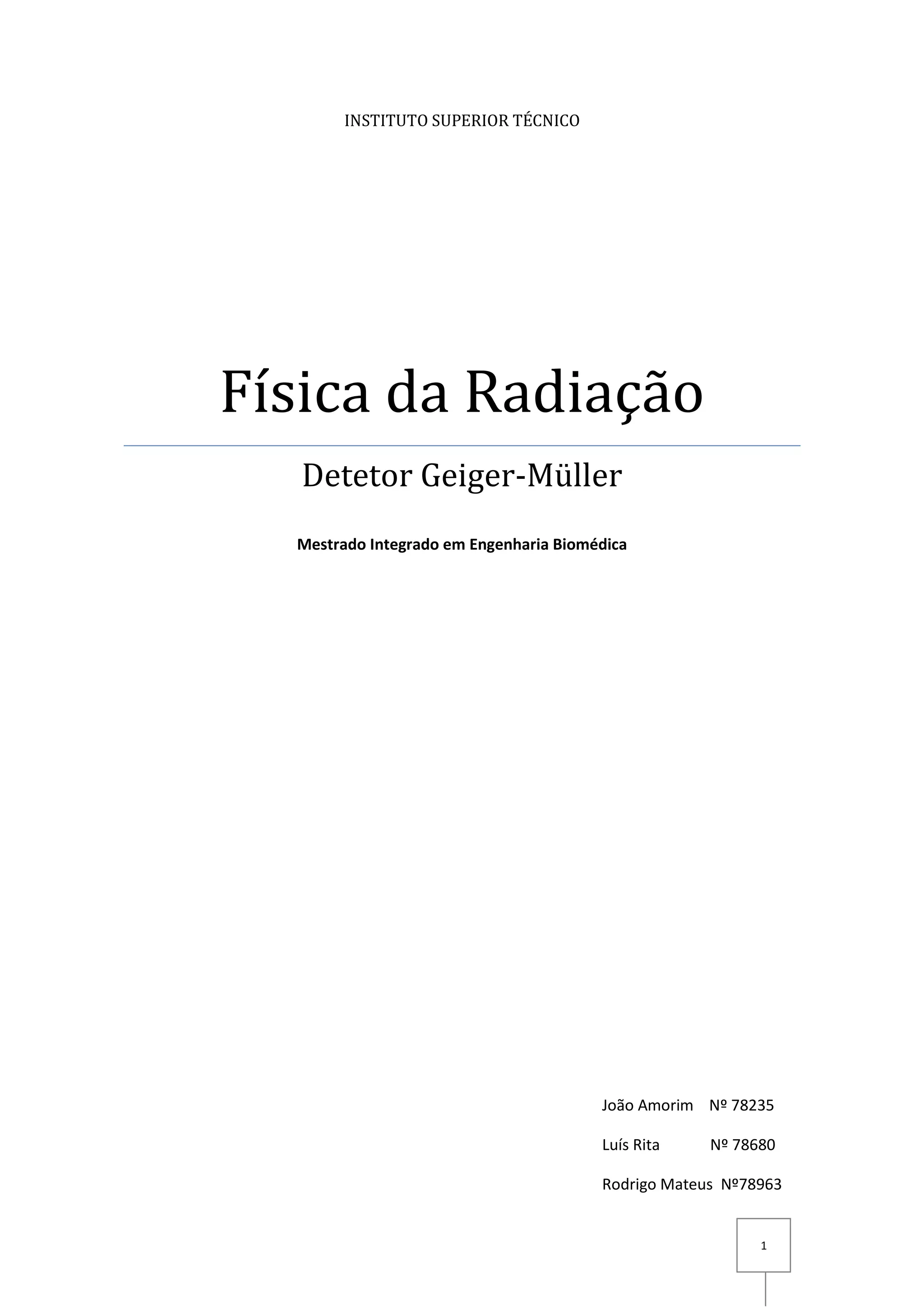
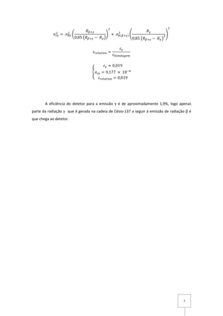
Foi construída a tabela 1, onde está registada a tensão aplicada, amplitude do sinal
observado no osciloscópio, o intervalo de tempo, o número de contagens e a taxa de
contagens. A contagem do número de desintegrações da fonte radioativa pode ser descrita
por uma distribuição de Poisson. De forma a que o erro estatístico no número de
contagens seja da ordem dos ε = 3 %, determinou-se o número de
contagens teórico adequado recorrendo à equação 1.
√ 𝑛
𝑛
=
1
√ 𝑛
= ε ⟺
⟺ 0.03 =
1
√ 𝑛
⟺ 𝑛 = 1111
A experiência foi iniciada com uma tensão de 500 V, mas como não foram obtidas
contagens, foi aumentada a tensão de 10 em 10 V até surgirem as primeiras contagens.
Depois, a tensão foi aumentada de 50 em 50 V.
O contador apresenta um limiar de tensão, abaixo do qual este não conta. Com o
decorrer da experiência verificámos este facto. O valor do limiar de tensão (em módulo) a
partir do qual o aparelho fazia contagens era 150 mV e por observação do sinal do osciloscópio
verificamos que o detetor só fazia contagens para sinais com amplitude superior a este mesmo
valor.
Tabela 1: Taxas de contagem, amplitudes de onda, intervalos de tempo e nº de contagens em
função da tensão aplicada. O patamar encontra-se definido no intervalo [600,900] V.
Tensão Aplicada (V) Amplitude (mV) ∆𝒕 (s) 𝑵 ± ∆𝑵 𝑹 ± ∆𝑹
(s-1
)
500 0,15 100,60 0 0
530 0,17 100,00 0 0
540 0,18 100,01 213 ± 15 2,13 ± 0,15
550 0,20 92,60 1214 ± 35 13,11 ± 0,38
600 0,22 87,02 1203 ± 35 13,82 ± 0,40
650 0,27 84,85 1206 ± 35 14,21 ± 0,42
700 0,30 83,21 1200 ± 35 14,42 ± 0,41
750 0,33 84,06 1200 ± 35 14,27 ± 0,38
800 0,36 86,05 1202 ± 35 13,97 ± 0,40
850 0,40 82,95 1203 ± 35 14,50 ± 0,42
900 0,44 83,18 1205 ± 35 14,49 ± 0,45
Notação
N – Nº de contagens;
R – Taxa de contagens;
R’ – Taxa de contagens sem fundo;

3. 3
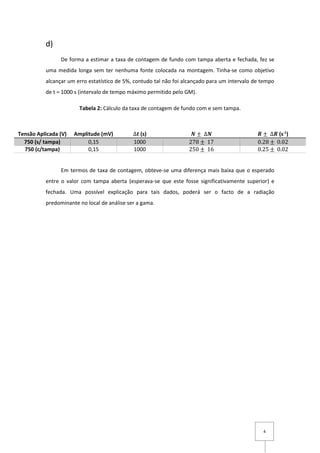
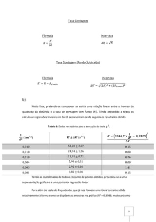
Figura 1: Curva da taxa de contagens em função da tensão aplicada.
Por análise do gráfico na figura 1, constata-se que o patamar se encontra entre os valores de
tensão 550 V e 950 V. Optou-se por uma tensão de trabalho de 750 V.
c)
Figura 2: Sinal observado no osciloscópio. O sinal tem uma amplitude de 0.27 V e uma duração
temporal de 130 µs. Devido ao funcionamento do detetor de Geiger-Müller o sinal chega a
atingir valores positivos após os 10 µs.
0
2
4
6
8
10
12
14
16
18
500 550 600 650 700 750 800 850 900 950 1000
TxadeContagem[s-1]
Amplitude [V]
Taxa de contagens em função da tensão aplicada

4. 4
d)
De forma a estimar a taxa de contagem de fundo com tampa aberta e fechada, fez se
uma medida longa sem ter nenhuma fonte colocada na montagem. Tinha-se como objetivo
alcançar um erro estatístico de 5%, contudo tal não foi alcançado para um intervalo de tempo
de t = 1000 s (intervalo de tempo máximo permitido pelo GM).
Tabela 2: Cálculo da taxa de contagem de fundo com e sem tampa.
Em termos de taxa de contagem, obteve-se uma diferença mais baixa que o esperado
entre o valor com tampa aberta (esperava-se que este fosse significativamente superior) e
fechada. Uma possível explicação para tais dados, poderá ser o facto de a radiação
predominante no local de análise ser a gama.
Tensão Aplicada (V) Amplitude (mV) ∆𝒕 (s) 𝑵 ± ∆𝑵 𝑹 ± ∆𝑹 (s-1
)
750 (s/ tampa) 0,15 1000 278 ± 17 0.28 ± 0.02
750 (c/tampa) 0,15 1000 250 ± 16 0.25 ± 0.02

5. 5
2. Estudo da Eficiência do Detetor para as Radiações 𝛽 e 𝛾
O estudo da eficiência do tubo de Geiger – Müller para estes dois tipos de radiação
pode ser realizado em primeira instância definindo uma configuração tal que as radiações β e
γ possam ser separadas, utilizando um princípio que indica que, enquanto a radiação γ é
bastante penetrante, a radiação β pode ser facilmente blindada.
Para tal utilizaram-se duas fontes radioativas, uma de Tálio ( 𝑇𝑙204
) e uma de Césio
( 𝐶𝑠137
), em experiências distintas e independentes, colocando as fontes sempre a 10 cm de
distância do tubo. De forma a ter sempre um erro estatístico relativo no número de contagens
entre 3% e 5%, apontou-se para o número de contagens ser igual a 1000.
a) De forma a obter apenas radiação β, utilizou-se a fonte de Tálio-204 e comparou-se a
taxa de contagens em duas situações - com a tampa da caixa aberta e com a tampa da
caixa fechada. Os resultados encontram-se apresentados na tabela abaixo.
Fonte Tampa ∆𝒕 (𝒔) 𝑵 + ∆𝑵 𝑹 + ∆𝑹 (𝒔−𝟏
) 𝑹′ ± 𝚫𝑹′ (𝒔−𝟏
)
𝑻𝒍𝟐𝟎𝟒
Aberta 70,49 1000 ± 32 14,12 ± 0,45 13,84 ± 0,45
𝑻𝒍𝟐𝟎𝟒
Fechada 1000 339 ± 18 0,34 ± 0,02 0,09 ± 0,01
Observando os valores da tabela acima, verificou-se que existe uma
disparidade bastante visível entre as contagens nos dois casos, razão pela qual
podemos inferir que o fecho da tampa da caixa resulta numa blindagem eficaz da
radiação β. É de referir que, à taxa de contagem total foi subtraída a taxa de contagem
do fundo e, no cálculo do erro, foi tido em conta a propagação dos erros. Teve-se
também em conta a radiação de fundo na situação com a tampa fechada é distinta da
presente com a tampa aberta. Calculou-se igualmente a eficiência da blindagem:
𝜀 𝑏𝑙𝑖𝑛𝑑𝑎𝑔𝑒𝑚 =
𝑅 𝑎𝑏𝑒𝑟𝑡𝑎 − 𝑅𝑓𝑒𝑐ℎ𝑎𝑑𝑎
𝑅 𝑎𝑏𝑒𝑟𝑡𝑎
=
14,12 − 0,34
14,12
= 0,976 ≈ 97,6 %
Tabela 3: Cálculo das taxas de contagem da fonte Tálio-204 para os casos de tampa aberta e tampa fechada.

6. 6
b)
𝑅 𝛽+𝛾 = 79,59 ± 2,49 contagens/s
c)
𝑅 𝛽+𝛾 = 79,31 ± 2,49 contagens/s
𝑅 𝛽+𝛾 = 𝑅 𝛾 + 𝑅 𝛽
𝑅 𝛾 = 1,26 ± 0,05 contagens/s
𝑅 𝛽 = 78,05 ± 2,49 contagens/s
d)
Na cadeia do Césio-137, quando ocorre declínio, a emissão de uma partícula 𝛽
é seguida da emissão de uma partícula γ em apenas 85% dos casos. Assim, a taxa de
contagem para a emissão de radiação γ é dada por:
𝑅 𝛾 = 0,85 𝑅 𝛽 = 66,34 ± 2,11 𝑐𝑜𝑛𝑡𝑎𝑔𝑒𝑛𝑠/𝑠
𝑅 𝛽 = 𝑅 𝛽+𝛾 − 𝑅 𝛾
𝜀 𝛾 =
𝑅 𝛾
𝑅 𝛾
0 =
𝑅 𝛾
0,85 𝑅 𝛽
0 =
𝑅 𝛾
0,85 (𝑅 𝛽+𝛾 − 𝑅 𝛾)
Fonte Tampa ∆𝒕 (𝒔) 𝑵 ± ∆𝑵 𝑹 ± ∆𝑹 (𝒔−𝟏
) 𝑹′ ± 𝚫𝑹′ (𝒔−𝟏
)
𝑪𝒔𝟏𝟑𝟕
Aberta ( β + γ ) 12,79 1018 ± 32 79,59 ± 2,49 79,31 ± 2,49
𝑪𝒔𝟏𝟑𝟕
Fechada ( γ) 660,69 1001 ± 32 1,51 ± 0,05 1,26 ± 0,05
Tabela 4: Cálculo das taxas de contagem da fonte Césio-137 para os casos de tampa aberta e tampa fechada.

7. 7
𝜎𝜀𝛾
2
= 𝜎 𝑅𝛾
2
(
𝑅 𝛽+𝛾
0,85 (𝑅 𝛽+𝛾 − 𝑅 𝛾)
)
2
+ 𝜎 𝑅(𝛽+𝛾)
2
(
𝑅 𝛾
0,85 (𝑅 𝛽+𝛾 − 𝑅 𝛾)
2)
2
𝜀 𝑟𝑒𝑙𝑎𝑡𝑖𝑣𝑎 =
𝜀 𝛾
𝜀 𝑏𝑙𝑖𝑛𝑑𝑎𝑔𝑒𝑚
{
𝜀 𝛾 ≈ 0,019
𝜎𝜀𝛾 = 9,177 × 10−4
𝜀 𝑟𝑒𝑙𝑎𝑡𝑖𝑣𝑎 = 0,019
A eficiência do detetor para a emissão γ é de aproximadamente 1,9%, logo apenas
parte da radiação γ que é gerada na cadeia de Césio-137 a seguir à emissão de radiação β é
que chega ao detetor.

8. 8
3. Estudo da lei de variação da taxa de contagem com a
distância do detetor à fonte
Introdução
A taxa de contagens no detetor GM, tal como se sabe, depende da intensidade da fonte
emissora, da eficiência do detetor para determinado tipo de radiação (determinada atrás) e
também da distância entre o detetor e a fonte. Na verdade, pode-se olhar para esta última
caraterística de 2 formas diferentes:
1. Este parâmetro é relevante, na medida em que a radiação é parcialmente absorvida
pela própria atmosfera. Quanto maior a distância, maior o grau de absorção.
2. Fração do ângulo sólido (do emissor de partículas) coberto pelo detetor. Ou seja,
quanto maior for a área do GM, maior será o nº de contagens (isto acontece porque
não se está a trabalhar com um feixe de radiação, mas sim, com uma fonte que emite
radiação em várias direções distintas.
a)
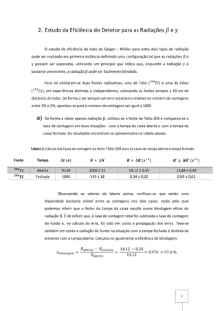
Nesta fase, voltou-se a utilizar a fonte de Tálio-204 e começou-se por determinar o
número de contagens e o intervalo de tempo associado à medição. Uma vez que se pretendia
que o erro fosse da ordem dos 5%, procedeu-se a, mais ou menos, 400 contagens. Tendo
concluído este passo, calculou-se a Taxa de Contagem e a Taxa de Contagem (Fundo
Subtraído). Bem como, as respetivas incertezas associadas, recorrendo às seguintes fórmulas:
𝒅 (𝒄𝒎) ∆𝒕 (𝒔) 𝑵 ± ∆𝑵 𝑹 ± ∆𝑹 (𝒔−𝟏
) 𝑹′ ± ∆𝑹′ (𝒔−𝟏
)
5 7,48 400 ± 20 53,48 ± 2,67 53,20 ± 2,67
7,5 15,98 403 ± 20 25,22 ± 1,26 24,94 ± 1,26
10 28,33 402 ± 20 14,19 ± 0,71 13,91 ± 0,71
15 63,80 400 ± 20 6,27 ± 0,31 5,99 ± 0,31
20 125,05 400 ± 20 3,20 ± 0,16 2,92 ± 0,16
30 362,67 400 ± 20 1,10 ± 0,06 0,82 ± 0,06
Tabela 5: Taxas de contagem, amplitudes de onda, intervalos de tempo e nº de contagens em função da tensão aplicada.
O patamar encontra-se definido no intervalo [600,900] V.

9. 9
Taxa Contagem
Taxa Contagem (Fundo Subtraído)
b)
Nesta fase, pretende-se comprovar se existe uma relação linear entre o inverso do
quadrado da distância e a taxa de contagem sem fundo (R’). Tendo procedido a todos os
cálculos e regressões lineares em Excel, representam-se de seguida os resultados obtido.
Tendo as coordenadas de todo o conjunto de pontos obtidos, procedeu-se a uma
representação gráfica e a uma posterior regressão linear.
Para além do teste do R-quadrado, que já nos fornece uma ideia bastante sólida
relativamente à forma como se dispõem as amostras no gráfico (R² = 0,9988, muito próximo
𝟏
𝒅 𝟐
(𝒄𝒎−𝟐
) 𝑹′ ± ∆𝑹′ (𝒔−𝟏
) 𝑹′
− (𝟏𝟑𝟒𝟒, 𝟕 ×
𝟏
𝒅 𝟐 − 𝟎, 𝟎𝟑𝟐𝟗)
𝟐
∆𝑹′
0,040 53,20 ± 2,67 0,15
0,018 24,94 ± 1,26 0,80
0,010 13,91 ± 0,71 0,26
0,004 5,99 ± 0,31 0,00
0,003 2,92 ± 0,16 1,41
0,001 0,82 ± 0,06 0,15
Incerteza
∆𝑅 = √𝑁
Fórmula
𝑅 =
𝑁
∆𝑡
Fórmula
𝑅′
= 𝑅 − 𝑅 𝐹𝑢𝑛𝑑𝑜
Incerteza
∆𝑅′ = √(∆𝑅)2 + (∆𝑅 𝐹𝑢𝑛𝑑𝑜)2
Tabela 6: Dados necessários para a execução do teste 𝜒2
.

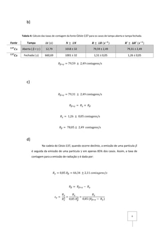
10. 10
de 1, ou seja, excelente ajuste), procedeu-se ao teste do 𝜒2
de forma a comprovar a relação
linear existente entre as 2 quantidades (R’ e
1
𝑑 𝟐).
.
Teste do 𝜒2
𝜒2
= 0,15 + 0,80 + 0,26 + 1,41 + 0,15 = 2,77
𝜒6
2
=
𝜒2
6
= 0,46
Estado em posse do valor "normalizado" , pode-se utilizar uma tabela [1] para
descobrir a probabilidade de se obter um valor igual ou superior a este. E, assim, afirmar com
que grau de certeza estarão os valores distribuídos segundo este modelo (linear). Neste caso,
para 6 graus de liberdade, pode-se afirmar com um grau de probabilidade superior a 99,5%
que os valores registados se relacionam pela seguinte expressão: y = 1344,7x - 0,0329.
Finalmente, tal como seria de esperar, observou-se que a taxa de contagens diminui
com a distância, por todas as razões discutidas na alínea a).
y = 1344,7x - 0,0329
R² = 0,9988
0
10
20
30
40
50
60
0 0,005 0,01 0,015 0,02 0,025 0,03 0,035 0,04 0,045
𝑹′
1/𝑑^2
Fórmula
𝜒2
= ∑
(𝑦𝑖 − 𝑦(𝑥𝑖))
2
𝜎2
𝑛
𝑖=1
Figura 3: Taxas de Contagem em Função do Inverso do Quadrado da Distância

11. 11
c)
Pelo esquema do declínio de 204
Tl, Qβ = 763.72 keV (figura 4). Observando a figura 5,
um valor de energia de partículas β próximo de 763 keV corresponde a um alcance de,
aproximadamente, 220 cm. Ou seja, para distâncias de algumas dezenas/unidades de cm (tal
como as utilizadas no trabalho), a absorção destas partículas não é suficientemente relevante.
Para além disto, verificou-se que a relação linear anterior se ajusta quase como
perfeitamente aos dados, conclui-se que, se houve uma atenuação, esta é desprezável para a
gama de distâncias utilizadas.
Figura 4: Decaimento do 204
Tl.
Figura 5: Alcance das partículas β no ar, em função da própria energia.

12. 12
d)
Até este ponto, apenas têm sido consideradas incertezas estatísticas associadas aos
valores apresentados anteriormente. No entanto, erros sistemáticos como: a colocação menos
correta do emissor e a paralaxe na leitura de instrumentos analógicos (medição da distância
entre fonte e detetor) podem ter contribuído para um afastamento dos resultados,
relativamente ao previsto.
De forma a obter uma estimativa da preponderância destes erros relativamente aos
estatísticos, realizaram-se 3 medições consecutivas (reposicionando a fonte antes de iniciar
cada uma). Apresenta-se de seguida uma tabela com os valores obtidos.
De seguida, procedeu-se ao cálculo de 𝐸(𝑅′) e 𝐸(𝑅′)2
de forma a poder estimar o desvio
padrão.
𝑅′̅̅̅ = 𝐸(𝑅′) =
14,00 + 13,83 + 13,87
3
= 13,90 𝑠−1
𝐸(𝑅′2) =
196,00 + 191,27 + 192,38
3
= 193,22 𝑠−1
𝜎 = √𝐸(𝑅′2) − 𝐸(𝑅′)2 = 0.07
Após a realização destes cálculos, é possível perceber que o erro sistemático associado
à posição da fonte é desprezável quando comparado com o estatístico (é menor numa ordem
de grandeza).
𝒅 (𝒄𝒎) ∆𝒕 (𝒔) 𝑵 ± ∆𝑵 𝑹′ ± ∆𝑹′ (𝒔−𝟏
)
10 27,87 398 ± 20 14,00 ± 0,72
10 28,99 409 ± 20 13,83 ± 0,69
10 28,33 401 ± 20 13,87 ± 0,71
Tabela 7: 3 medições efetuadas a distâncias semelhantes, de forma a atestar a relevância de um erro sistemático.