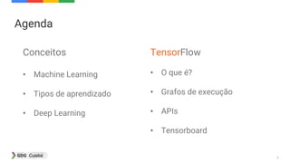
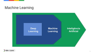
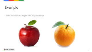
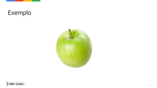
Transferir como PDF, PPTX


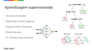
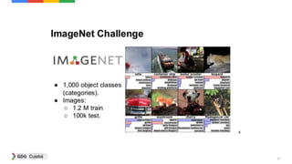
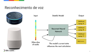
![14
from sklearn import datasets, svm, metrics
import matplotlib.pyplot as plt
# Carrega o dataset
digits = datasets.load_digits()
# transforma a imagem em vetor
n_samples = len(digits.images)
data = digits.images.reshape((n_samples, -1))
x_train = data[:n_samples / 2]
y_train = digits.target[:n_samples / 2]
# cria um classificador SVM
classifier = svm.SVC(gamma=0.001)
# realiza o ajuste dos dados
classifier.fit(x_train, y_train)
esperado = digits.target[n_samples / 2:]
predito = classifier.predict(data[n_samples / 2:])](https://image.slidesharecdn.com/apresentacao-170326185253-170326213340/85/Introducao-a-Machine-Learning-e-TensorFlow-14-320.jpg)
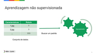
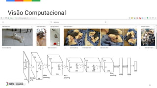
![16
import matplotlib.pyplot as plt
from sklearn.cluster import KMeans
from sklearn.datasets import make_blobs
n_samples = 1500
random_state = 170
X, y = make_blobs(n_samples=n_samples, random_state=random_state)
y_pred = KMeans(n_clusters=3, random_state=random_state).fit_predict(X)
plt.subplot(211)
plt.scatter(X[:, 0], X[:, 1], c=y_pred)
plt.title("Iniciado com 3 centroides")
y_pred = KMeans(n_clusters=2, random_state=random_state).fit_predict(X)
plt.subplot(212)
plt.scatter(X[:, 0], X[:, 1], c=y_pred)
plt.title("Iniciado com 2 centroides")
plt.show()](https://image.slidesharecdn.com/apresentacao-170326185253-170326213340/85/Introducao-a-Machine-Learning-e-TensorFlow-16-320.jpg)
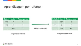

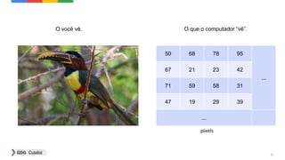
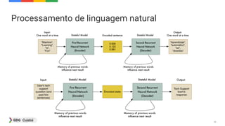
![22
import numpy as np
import keras
from keras.preprocessing import image
from keras.applications.inception_v3 import preprocess_input,
decode_predictions
model = keras.applications.InceptionV3(weights='imagenet')
img_path = 'aracari_castanho.jpg'
img = image.load_img(img_path, target_size=(299,299))
x = image.img_to_array(img)
x = np.expand_dims(x, axis=0)
x = preprocess_input(x)
preds = model.predict(x)
# decode
print('Predicted:', decode_predictions(preds, top=3)[0])
Toucan 71,27%
Hornbill 16,84%
School Bus 1,65%
Predicted: [('n01843383', 'toucan', 0.71278381), ('n01829413', 'hornbill', 0.16843531), ('n04146614', 'school_bus', 0.01657751)]](https://image.slidesharecdn.com/apresentacao-170326185253-170326213340/85/Introducao-a-Machine-Learning-e-TensorFlow-22-320.jpg)
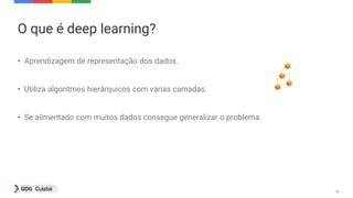
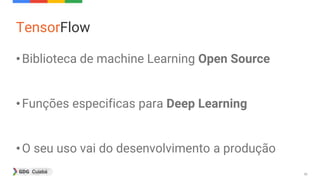
![23
import numpy as np
import keras
from keras.preprocessing import image
from keras.applications.inception_v3 import preprocess_input,
decode_predictions
model = keras.applications.InceptionV3(weights='imagenet')
img_path = 'arvore.jpg'
img = image.load_img(img_path, target_size=(299, 299))
x = image.img_to_array(img)
x = np.expand_dims(x, axis=0)
x = preprocess_input(x)
preds = model.predict(x)
# decode
print('Predicted:', decode_predictions(preds, top=3)[0])
Lakeside 21,76%
Church 8,03%
Valley 7,81%
Predicted: [('n09332890', 'lakeside', 0.21762265), ('n03028079', 'church', 0.080397919), ('n09468604', 'valley', 0.078168809)]](https://image.slidesharecdn.com/apresentacao-170326185253-170326213340/85/Introducao-a-Machine-Learning-e-TensorFlow-23-320.jpg)
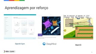
![24
import numpy as np
import keras
from keras.preprocessing import image
from keras.applications.inception_v3 import preprocess_input,
decode_predictions
model = keras.applications.InceptionV3(weights='imagenet')
img_path = 'alvaro.jpg'
img = image.load_img(img_path, target_size=(299, 299))
x = image.img_to_array(img)
x = np.expand_dims(x, axis=0)
x = preprocess_input(x)
preds = model.predict(x)
# decode
print('Predicted:', decode_predictions(preds, top=3)[0])
Jersey 51,26%
Wig 2,58%
Drumstick 2,12%
Predicted: [('n03595614', 'jersey', 0.51262307), ('n04584207', 'wig', 0.025850503), ('n03250847', 'drumstick', 0.021243958)]](https://image.slidesharecdn.com/apresentacao-170326185253-170326213340/85/Introducao-a-Machine-Learning-e-TensorFlow-24-320.jpg)


![39
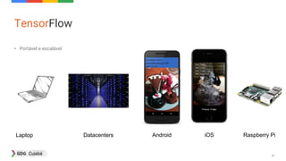
• Vetor n-dimensional, onde n = [0, 1, 2, 3, ...]
Escalar S = 42
Vetor V = [1, 2, 3, 4]
Matriz M = [[1, 0],[0, 1]]
Cubo ...](https://image.slidesharecdn.com/apresentacao-170326185253-170326213340/85/Introducao-a-Machine-Learning-e-TensorFlow-39-320.jpg)


![49
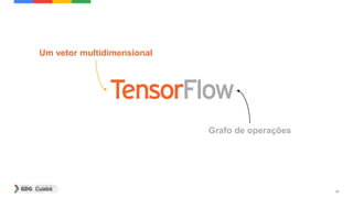
Low Level API
import tensorflow as tf
from tensorflow.contrib.learn.python.learn.datasets.mnist import read_data_sets
mnist = read_data_sets("MNIST_data/", one_hot=True)
def create_layer(name, x_tensor, num_outputs):
shape = x_tensor.get_shape().as_list()[1:]
with tf.name_scope(name):
weights = tf.Variable(tf.random_normal([shape[0], num_outputs], stddev=0.1), name='Weights')
bias = tf.Variable(tf.zeros(num_outputs), name='biases')
fc = tf.add(tf.matmul(x_tensor, weights), bias)
fc = tf.nn.relu(fc)
tf.summary.histogram('histogram', fc)
return fc
sess = tf.InteractiveSession()](https://image.slidesharecdn.com/apresentacao-170326185253-170326213340/85/Introducao-a-Machine-Learning-e-TensorFlow-49-320.jpg)
![50
Low Level API
x = tf.placeholder(tf.float32, shape=[None,784])
y_ = tf.placeholder(tf.float32, shape=[None,10])
with tf.name_scope('dnn'):
h0 = create_layer('hidden_0', x, 32)
h1 = create_layer('hidden_1', h0, 128)
h2 = create_layer('hidden_2', h1, 32)
with tf.name_scope('logit'):
W = tf.Variable(tf.zeros([32, 10]), name='weights')
b = tf.Variable(tf.zeros([10]),name='biases')
y = tf.matmul(h2,W) + b
tf.summary.histogram('histogram', y)
cross_entropy = tf.reduce_mean(tf.nn.softmax_cross_entropy_with_logits(logits=y, labels=y_))](https://image.slidesharecdn.com/apresentacao-170326185253-170326213340/85/Introducao-a-Machine-Learning-e-TensorFlow-50-320.jpg)
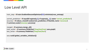
![52
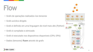
Low Level API
for i in range(2000):
if i%10 ==0:
summary, acc = sess.run([merged, accuracy],feed_dict={x: mnist.test.images, y_: mnist.test.labels})
test_writer.add_summary(summary,i)
print('Step: {}, Accuracy: {}'.format(i,acc))
else:
batch = mnist.train.next_batch(100)
summary, _ = sess.run([merged, train_step], feed_dict={x: batch[0], y_: batch[1]})
train_writer.add_summary(summary, i)
print(accuracy.eval(feed_dict={x: mnist.test.images, y_: mnist.test.labels}))
Acurácia final: 0.9645](https://image.slidesharecdn.com/apresentacao-170326185253-170326213340/85/Introducao-a-Machine-Learning-e-TensorFlow-52-320.jpg)
![53
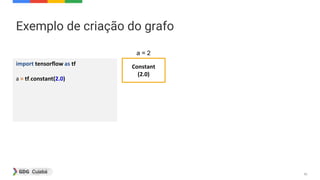
High Level API
def generate_input_fn(dataset, batch_size=BATCH_SIZE):
def _input_fn():
X = tf.constant(dataset.images)
Y = tf.constant(dataset.labels.astype(numpy.int64))
image_batch, label_batch = tf.train.shuffle_batch([X,Y], batch_size=batch_size, capacity=8*batch_size,
min_after_dequeue=4*batch_size, enqueue_many=True)
return {'pixels': image_batch} , label_batch
return _input_fn
mnist = read_data_sets("MNIST_data/", one_hot=False)
feature_columns = [tf.contrib.layers.real_valued_column("pixels", dimension=784)]
classifier = tf.contrib.learn.DNNClassifier(feature_columns=feature_columns, hidden_units=[32, 128, 32],
n_classes=10, model_dir="/tmp/mnist_model_2")
classifier.fit(input_fn=generate_input_fn(mnist.train, batch_size=100), steps=2000)
accuracy_score = classifier.evaluate(input_fn=generate_input_fn(mnist.test, batch_size=100), steps=2000)['accuracy']
print('DNN Classifier Accuracy: {0:f}'.format(accuracy_score))
DNN Classifier Accuracy: 0.9635](https://image.slidesharecdn.com/apresentacao-170326185253-170326213340/85/Introducao-a-Machine-Learning-e-TensorFlow-53-320.jpg)
![54
Keras
from keras.models import Sequential
from keras.layers import Dense
from keras.optimizers import RMSprop
from tensorflow.contrib.learn.python.learn.datasets
.mnist import read_data_sets
mnist = read_data_sets("MNIST_data/", one_hot=True)
batch_size = 100
epochs = 20
x_train, y_train = mnist.train.next_batch(50000)
x_test, y_test = mnist.test.next_batch(10000)
model = Sequential()
model.add(Dense(32, activation='relu', input_shape=(784,)))
model.add(Dense(128, activation='relu'))
model.add(Dense(32, activation='relu'))
model.add(Dense(10, activation='softmax'))
model.summary()
model.compile(loss='categorical_crossentropy',
optimizer=RMSprop(),
metrics=['accuracy'])
history = model.fit(x_train, y_train, batch_size=batch_size,
verbose=1, validation_data=(x_test, y_test))
score = model.evaluate(x_test, y_test, verbose=0)
print('Test loss:', score[0])
print('Test accuracy:', score[1])
Test accuracy: 0.9685](https://image.slidesharecdn.com/apresentacao-170326185253-170326213340/85/Introducao-a-Machine-Learning-e-TensorFlow-54-320.jpg)


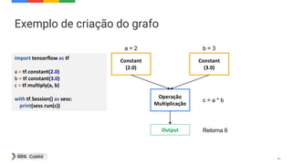
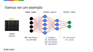
[1] Este documento introduz conceitos de machine learning e TensorFlow, incluindo tipos de aprendizado, deep learning e como TensorFlow funciona com grafos de execução e APIs. [2] É apresentado um exemplo de classificação de imagens usando redes neurais com TensorFlow e Keras para demonstrar estas técnicas. [3] Referências adicionais sobre estes tópicos são fornecidas no final.


![[Ahirton Lopes e Rafael Arevalo] Deep Learning - Uma Abordagem Visual](https://cdn.slidesharecdn.com/ss_thumbnails/ahirtonlopeserafaelarevalodeeplearning-umaabordagemvisual-190215183628-thumbnail.jpg?width=640&height=640&fit=bounds)
![[Jose Ahirton Lopes] Deep Learning - Uma Abordagem Visual](https://cdn.slidesharecdn.com/ss_thumbnails/joseahirtonlopesdeeplearning-umaabordagemvisual-181209205137-thumbnail.jpg?width=640&height=640&fit=bounds)
![[Jose Ahirton Lopes] Deep Learning - Uma Abordagem Visual](https://cdn.slidesharecdn.com/ss_thumbnails/joseahirtonlopesdeeplearning-umaabordagemvisual-181204182142-thumbnail.jpg?width=640&height=640&fit=bounds)
![[Jose Ahirton lopes] Do Big ao Better Data](https://cdn.slidesharecdn.com/ss_thumbnails/ahirtonlopesdobigaobetterdata-190410143141-thumbnail.jpg?width=640&height=640&fit=bounds)

![[Jose Ahirton Lopes] Inteligencia Artificial - Uma Abordagem Visual](https://cdn.slidesharecdn.com/ss_thumbnails/joseahirtonlopesinteligenciaartificial-umaabordagemvisual-200103185454-thumbnail.jpg?width=640&height=640&fit=bounds)

![[Jose Ahirton Lopes] Inteligencia Artificial - Uma Abordagem Visual](https://cdn.slidesharecdn.com/ss_thumbnails/joseahirtonlopes-meetupinteligenciaartificial-umaabordagemvisual-200215025106-thumbnail.jpg?width=640&height=640&fit=bounds)
