Trabalho final da disciplin ade Remote Sensing, UNL, 2007

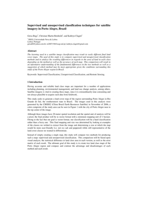
1. Supervised and unsupervised classification techniques for satellite
imagery in Porto Alegre, Brazil
Geisa Bugs1, Christian Martin Reinhold1, and Kathryn Clagett1
1
ISEGI, Universidade Nova de Lisboa
Lisboa, Portugal
geisa80@yahoo.com.br; m2007158@isegi.unl.pt; kathryn.clagett@gmail.com
Abstract
The learning used in a satellite image classification may result in vastly different final land
cover maps. The goal of this study is to compare supervised and unsupervised classification
methods and to analyze the resulting differences in regards to the area of land in each class
depending on the method as well as the accuracy of each map. This comparison will result in
an informative understanding of the fundamental differences in the two methods as well as a
suggestion of which method may be most appropriate given the conditions surrounding this
study of the Porto Alegre region in Brazil.
Keywords: Supervised Classification, Unsupervised Classification, and Remote Sensing.
1 Introduction
Having accurate and reliable land class maps are important for a number of applications
including planning, environmental management, and land use change analysis, among others.
Satellite imagery is vital to creating these maps, since it is extraordinarily time consuming and
not always plausible to acquire such data from fieldwork.
This study seeks to generate a land cover map of the region surrounding Porto Alegre in Rio
Grande do Sul, the southernmost state in Brazil. The images used in this analysis were
generated by the CBERS2 (China Brazil Earth Resources Satellite) in November of 2006; a
color composite of the study area can be seen in Figure 1 with the city of Porto Alegre near to
the top center of the image.
Although these images have 20-meter spatial resolution and the spatial unit of analysis will be
a pixel, the final product will be in vector format with a minimum mapping unit of 1 hectare.
Owing to the fact that our goal is vector format, our classification will be a hard classification
rather than a fuzzy one. This final mapping unit size was determined by looking at examples
of the classes we wished to extract from the image and determining a size at which the map
would be more user-friendly (i.e. not too salt and peppered) while still representative of the
land cover classes we wanted to differentiate.
Instead of simply creating a single map, this study will compare two methods for producing
such a map: supervised and unsupervised classification. This comparison will be based upon
visual analysis, the statistical difference in land class area in each version, as well as the error
matrix of each result. The ultimate goal of this study is to create two land class maps of the
Porto Alegre region and compare and contrast the advantage and disadvantages of each
method and each result.

2. Figure 1: color composite of the study area in southern Brazil (from CBERS2, using green, red,
and near infrared bands).
2 Study area and dataset
This section will cover not only the physical study area on the ground but also the study area in
regards to the images used in processing.
2.1 Porto Alegre region
With a population in the city of about 1.4 million, Porto Alegre is the capital of Rio Grande do
Sul, a state in the south of Brazil. The city is centered around 30°01’59’’ south latitude and
51°13’48’’ west longitude and has an area of approximately 500 km2. We chose to look not
just at the city itself but also its surroundings due to the fact that this provides an interesting
example for remote sensing because of the diversity of landscape this area represents; while
the city is a thriving metropolis, this image also shows many smaller farm regions and hamlets
in the countryside.
2.2 CBERS2 image
As discussed before, this image is from the China Brazil Earth Resources Satellite and, more
specifically, from the CCD (charge-coupled device) sensor. The CCD sensor is multi-spectral,
providing images at a 20m by 20m resolution with five bands: band 1 is a blue band from .45-
.52mµ; band 2 a green band from .52-.59 mµ; band 3 a red band from .63-.69 mµ; band 4 a
near infrared band from .76-.89 mµ; and band 5 a panchromatic band from .51-.73µ. The
temporal resolution of this sensor is 26 days. Because we had access to a number of high
resolution images from November that could be used both in gathering the training sites and
accuracy assessment, we chose an image from November, in this case November of 2006
which was taken at 11:13 am Brazilian time; this image’s ID number is

3. CBERS_2_CCD_1XS_2006_1123_157_134_L2. The study area is also 113 kilometers on
each side and comes pre-projected in the South American Datum 1969 for UTM zone 21S.
Lastly, the image come geometrically corrected using cubic convolution, where each pixel’s
digital number is actually an average of its surrounding pixels.
3 Methodology
This section will review the classification nomenclature used, the feature selection process,
preprocessing, classification method, and post-processing in turn. Due to the landscape of our
study area and the spatial unit of analysis we opted out of any image stratification or
segmentation for this study.
3.1 Classification nomenclature
Since it can be useful to use an established classification system in order be able to more
widely apply and compare the results of a land class map, we attempted to use the USGS Land
Use/Land Cover Classification System for our classification purposes. However, we also
wanted to be able to represent the specific landscape features of this area well, so we
additionally turned to existing land class maps of various parts of the area represented in the
image. Combining these systems, we were able to come up with eight classes that represent
the land cover of the Porto Alegre region well; these are presented in Table 1. To ensure that
our classes account for all possible types of landscape, we used the Land Cover Classification
System software to double-check that the classes we created represented every possible part of
the landscape.
Table 1: Classification nomenclature and description.
Class Description
1 Urban Built-up and mixed urban land use (residential, commercial, industrial, etc)
2 Fields Pasture, grassland, <20% sparse vegetation, rangeland
3 Natural Forest Areas with >60% crown cover vegetation
4 Regrowth Forest Areas with 20-60% crown cover vegetation
5 Agriculture Cropland, orchards, groves
6 Water Lakes, rivers, canals, dams (>30% water)
7 Wetland Areas with <30% water
8 Beach Sandy areas
3.2 Pre-processing
Preprocessing encompasses any geometric or radiometric correction that you need to do before
processing your image. In our case, as mentioned, the image came geometrically corrected by
INPE (Instituto Nacional de Pesquisas Espaciais), the organization that provides the satellite
images, through the cubic convolution method. Likewise, radiometric correction was deemed
unnecessary for this image; radiometric correction is only a necessity when doing
multitemporal analysis, quantitative analysis, or when the study area has significant
topography that might lead to the over or underestimation of digital numbers. Since none of
these conditions were a part of our analysis, as with geometric correction, we did not have to
worry about radiometrically correcting the image.

4. 3.3 Feature selection
As mentioned, we had four bands to work with for the purposes: blue, green, red, and near
infrared. Our first attempts were to use all four bands in our analysis. However, due to
technical problems, we were ultimately not able to use the blue band in the analysis. This
limited us to the other three bands and we used all three of them in our analysis. Because of
the tendency for urban areas and certain types of agriculture to have similar digital numbers,
we decided to also employ a texture analysis to one of the bands in an attempt to retrieve better
results; this type of analysis has been shown to greatly improve the outcome of a land class
analysis (Lu and Weng, 2007). To create this texture, the ‘filter’ tool in ArcGIS was used, at a
‘low’ setting on the near infrared band. This image was then included in the analysis in an
attempt to specifically better differentiate urban and agricultural land.
3.4 Classification method
The goal of our study is not simply to create a single classification map, but also to compare
two learning methods—supervised and unsupervised—by undertaking both types of analysis
on the image.
3.4.1 Supervised classification
The main difference between a supervised and unsupervised classification is the use (or non-
use, in the case of the latter) of training sites. For the supervised classification our goal was to
collect at least thirty training sites per class since it is suggested that you need at least 10n
training sites per class where n is the number of features to be used in the analysis (Jensen,
1996). These sites were collected using a combination of sources: personal knowledge of the
area, existing land cover maps for the area, Google Earth, and the aerial photographs that we
had access to. As a general rule we tried to have our training sites be as homogeneous as
possible in the class they represented while also providing a variety of different types of land
within that class throughout the whole image. Our training sites also were always larger than
one pixel in area. Both the homogeneity and variety of the training sites as well as their size
were chosen in hope of obtaining as accurate a mean vector for this class as possible. Without
getting into the results too much, our first attempts at classifying proved less than ideal so the
training sites used were revisited, altered, and added to in an effort to yield better results.
Supervised classifications using as few as 240 sites and as many as over 550 were run to figure
out which training site file was the most appropriate.
For the actual classification, the first step was to use the training sites we had found to create
signatures in ArcGIS. Maximum likelihood was used as the classification algorithm and with
this we input the signatures we had created. Since this algorithm works with probabilities,
treating every point as having an equal likelihood of belonging to any class, we had the
opportunity to include weights to help the classification; however, we opted to let the classifier
run without any additional weights. The maximum likelihood classifier is advantageous
because it works with probabilities so that high correlation in bands with classes is less
problematic and because it classifies every pixel in an image, which suits our purpose.
3.4.2 Unsupervised classification
In the unsupervised classification, we began the analysis with running the images through the
ISOcluster tool. This tool creates a specified number of spectral classes from the images that
are input. In our case, aiming to have 8 final classes, we asked the ISOcluster tool to create
thirty-six spectral classes. The result of this tool is a signature file like created with the

5. training samples that could be input again into the maximum likelihood tool. From this we
went through and reclassed these thirty-six spectral classes to informational classes by visually
analyzing the types of land each class represented. Because we were able to assign every
spectral class to an information class, we did not find it necessary to do any cluster busting
where we would further break down a spectral class into spectral sub-classes. Doing this we
were able to satisfactorily generate an unsupervised land cover map.
3.5 Post-processing
Because of our goal to ultimately create a vector map with a minimum mapping unit of one
hectare, we needed to generalize our image. The first step in doing this was to run several
majority filters on the raster maps for both the supervised and unsupervised classifications,
first with four neighbors and later with eight. This was necessary because in order to convert
to vector and eliminate the polygons with less than one hectare area we could not have too
many polygons—after our initial majority filter runs, the vector conversion resulted in over
one million polygons for the unsupervised classification, something that the computer did not
have enough memory to process.
Ultimately, when the majority filter had been run an adequate number of times, the vector
conversion of both the supervised and unsupervised images resulted in about 300,000
polygons. In order to generalize the polygons with an area less than one hectare, the eliminate
function was used in ArcGIS. The eliminate function has two options, either to eliminate to
the adjacent polygon with whom it shares the longest edge or with the adjacent polygon that
has the largest area, we made use of the second option. This tool was used first to eliminate
polygons with an area of less that .1 hectare, then .25, then .5, and finally one hectare. In
between each phase the areas were recalculated. The logic behind this incremented approach
was that after the first elimination, perhaps two smaller polygons would be merged resulting in
an area larger than 1 hectare, whereas if you immediately eliminate all polygons with an area
less than one hectare, you will skip ahead to a much grosser generalization. Using majority
filter and polygon elimination in ArcGIS allows for us to create our final product, two
classification maps for land cover in the Porto Alegre region, one for supervised classification
and another for unsupervised classification, both of which are in vector format and have a final
minimum mapping unit of one hectare.
4 Results
The results of the two mapping classifications are presented in Figures 2 and 3, both in their
raster form before generalization and in their final vector form. Clearly there are some major
differences in the two maps. Interestingly, these differences seem less apparent with the raster
images—generalization seems to heighten the variation between the two. The exact
significance of the differences between the two maps will be addressed in the discussion
section.
The accuracy assessments of the final vector-based maps for the supervised and unsupervised
classifications are presented in Tables 2 and 3. The accuracy assessment was done by
manually choosing approximately fifty pixels per class and assigning them the class they
represent in ‘real life’—these pixels were chosen to be as spread out and as representative of
the class as possible while still being clearly one class. The overall accuracy for the supervised
classification was 76% while the overall accuracy for the unsupervised classification was
around 48%. Working off the idea that a good accuracy would be about 85%, it is clear that

6. neither of our maps really makes the grade; however, the accuracy of the supervised
classification is considerable higher than that of the unsupervised.
Table 2: Error matrix for supervised classification.
Natural Regrowth ROW User´s
Urban Fields Forest Forest Agriculture Water Wetland Beach TOTAL Accuracy
Urban 46 1 0 1 4 1 0 16 69 66.7%
Fields 0 32 0 2 6 0 15 0 55 58.2%
Natural
Forest 0 1 42 0 0 0 0 0 43 97.7%
Regrowth
Forest 0 0 3 46 0 0 0 0 49 93.9%
Agriculture 5 2 0 0 35 5 7 0 54 64.8%
Water 0 0 0 0 0 46 0 0 46 100.0%
Wetland 0 14 7 1 7 0 28 0 57 49.1%
Beach 0 0 0 0 0 0 0 35 35 100.0%
COLUMN
TOTAL 51 50 52 50 52 52 50 51 408
Producer´s
Accuracy 90.2% 64.0% 80.8% 92.0% 67.3% 88.5% 56.0% 68.6% 76.0%
Table 3: Error matrix for unsupervised classification.
Natural Regrowth ROW User´s
Urban Fields Forest Forest Agriculture Water Wetland Beach TOTAL Accuracy
Urban 33 12 1 1 3 0 0 0 50 66.0%
Fields 0 18 4 8 17 0 3 0 50 36.0%
Natural
Forest 0 0 26 10 8 5 0 0 49 53.1%
Regrowth
Forest 0 6 13 23 8 0 0 0 50 46.0%
Agriculture 8 15 0 0 26 0 1 0 50 52.0%
Water 1 0 0 2 2 43 0 1 49 87.8%
Wetland 1 6 10 5 21 2 5 0 50 10.0%
Beach 12 1 0 4 16 0 17 50 34.0%
COLUMN
TOTAL 55 58 54 49 89 66 9 18 398
Producer´s
Accuracy 60.0% 31.0% 48.1% 46.9% 29.2% 65.2% 55.6% 94.4% 48.0%

7. Figure 1: Initial raster (left) and final vector map (right) for supervised classification after generalizing and eliminating polygons less than one hectare.

8. Figure 2: Initial raster (left) and final vector map (right) for unsupervised classification after generalizing and eliminating polygons less than one hectare.

9. 5 Discussion
The discussion of our results will be broken down by our overall satisfaction and general
considerations for this study before exploring a comparison of the two methods and ultimately
looking at ways that our work could have been improved.
5.1 Overall evaluation
As the accuracy assessments show, both the supervised and unsupervised maps have
significant problems in representing what is actually happening on the ground. Interestingly,
with both methods, wetlands, fields, and agriculture had the lowest accuracy rate for both
producer’s and user’s accuracy. Problems in defining these categories likely come from the
close spectral relationship between pixels in these vegetated classes. Alternately or
additionally, the confusion between these classes may also stem from the incorrect placement
of training sites in the case of the supervised classification or the inappropriate assigning of
spectral classes in the unsupervised classification. Furthermore, these images are taken in
November, at the end of the rainiest part of the year in this region. This means that vegetation
would be thriving in most every type of land and this may lead to incorrectly assigning training
sites or problems in differentiating spectral classes of variant types of land class.
On the other end of the figurative spectrum, both methods were (not surprisingly) quite good at
distinguishing water and beach from the other classes. These two classes lie at either end of
the literal spectrum and therefore are less likely to be confused with other classes. In the
middle ground between wetland/fields/agriculture and beach/water are urban, natural forest,
and regrowth forest. The supervised classification actually distinguished the two types of
forest quite well while the results were not as good for the unsupervised. For the urban class,
there was a different situation altogether; in the supervised classification the producer’s
accuracy was very good, meaning that those pixels on the ground that were urban were classed
as urban while the user’s accuracy was quite low, while in the unsupervised classification, the
user’s accuracy was slightly better, meaning that those pixels classes as urban were in fact
urban and the producer’s accuracy was lower. Overall, it can be concluded that some of the
classes, those that tend to have a very unique range of digital numbers (beach and water), were
well classed while those whose spectral range is harder to distinguish had poorer results,
leading to generally mixed results for both final maps.
Since both of our maps were generalized several times, using equally the majority filter and
with the vector-based eliminate function, it is informative to compare the results from before
the generalization took place to those from after. You might assume, since these methods of
generalization reduce the number of distinct pixels for the sake of a larger minimum mapping
unit, that the error matrices from before the generalization would be higher than those from
after and, in fact, this is the case. While the entire accuracy matrices for the pre-generalization
images are not included here, the overall accuracy for the supervised classification is 77% for
before generalization (as compared with 76% for after) and almost 57% before for
unsupervised (as compared with 48% after). The overall accuracy of the supervised method
remains fairly constant while the overall accuracy of the unsupervised classification changes
significantly.
Even though overall supervised classification apparently doesn’t change that much after
generalization for the supervised method, Table 4 shows that in fact there is significant change
category to category from before generalization to after. Interestingly, a class likes wetland,

10. which has fairly bad overall accuracy, changes very little from before to after generalization.
Alternately, urban, which, relatively speaking, has higher accuracies than most of the other
classes, changes significantly. Likewise, beach and water, the other two categories with higher
general accuracy, have significant change from before and after generalization. Cleary, the
generalization of the images significantly alters the accuracy of different categories, bettering
some and worsening others, which may not be apparent from only looking at the change in
overall accuracy, which, for supervised classification, was only 1%.
Table 4: Difference in accuracies from before generalization to after.
Natural Regrowth
Urban Fields Forest Forest Agriculture Water Wetland Beach
Difference in - -
Supervised 23.5% 5.8% -16.9% -1.9% -2.7% 11.5% 2.2% 31.4%
Producer's Difference in -
Accuracy Unsupervised 7.6% -6.7% -18.5% -19.7% -7.6% 32.8% 0.0% -5.6%
Difference in
Supervised -25.3% -5.8% 12.0% 1.9% -5.2% 6.1% -6.9% 31.4%
User's Difference in - -
Accuracy Unsupervised -22.0% -4.0% -20.4% -6.0% -4.0% 10.2% -10.0% 17.0%
5.2 Comparison of supervised and unsupervised methods
A simple visual comparison of the results of the two methods for classification (Figures 2 and
3) reveal large differences in the result created by each image. These differences are
reinforced by Figure 4 that presents the percent area of each land class with each method in the
study area. For the urban, water, and beach categories, the percent area in each map is fairly
similar. The greatest differences, which are also visually apparent, are with agriculture and
wetland. Out of these, wetland has by far the largest difference, with vastly more wetland in
the supervised classification than in the unsupervised. Interestingly, wetland has fairly low
accuracy across the board, suggesting that despite the two methods providing such different
results, in fact neither is particularly correct—possibly the unsupervised classification is
underestimating the amount of wetland while the supervised classification is overestimating it.
By far the most important determinant of which methodology is preferable is the accuracy
assessment. While neither is ideal, the accuracy for the supervised classification is far superior
to that of the unsupervised. This fact is not surprising considering that with the supervised
classification training sites are used that have been hand-picked to determine the classes.
Overall, this study seems to confirm our suspicions that the supervised has better results than
the unsupervised. Ultimately, while it is true that the unsupervised method may save time
money in a project, in this case the results were only approximately 50% reliable; suggesting
that the time saved may not be worth the sacrifice.

11. 40%
35%
30%
25%
Super %
20%
Unsuper %
15%
10%
5%
0%
re
r
st
s
n
nd
st
ch
te
ld
ba
re
re
tu
a
tla
wa
fie
be
fo
fo
ur
ul
we
ric
th
l
ra
ow
ag
tu
na
gr
re
class
Figure 3: Comparison of areas of different classes of land for supervised and unsupervised
classification.
5.3 Improvements
While decently satisfactory results were achieved with the supervised classification, it is
always important to consider ways in which these results could be improved upon.
First off, there seems to be considerable mixing in the various vegetated classes. While it
could be that more, and more precise, training sites may be beneficial to distinguishing these
classes, our attempts at using additional training sites did not prove particularly productive.
Perhaps the best solution would to include different additional classes by which to differentiate
types of land. For example, in the supervised classification, hilltops just to the southeast of the
city of Porto Alegre are classes as wetland when in fact they are rocky fields. Due to their
makeup, the digital numbers for these fields may be lower than that of most of the other fields
that were primarily grassy. This means that perhaps the classifiers were not able to group
these fields properly. Creating two different categories for different types of fields may help
the results. Likewise, for the unsupervised classification, perhaps starting with more than 36
clusters would help differentiate this mixing in vegetation types.
Likewise, it could help to generate objects first, and then apply a decision tree model to those
objects to generate a class for each object. In fact, our initial hope was to create objects for
this assessment, however, technical difficulties made this impossible. Creating objects would
likely reduce our need to generalize in order to obtain our desired minimum mapping unit and
therefore perhaps prevent the loss of accuracy that we discovered as we generalized out
outputs for the final map.
Furthermore, while we ran a four-neighbor generalization four times and then an eight-
neighbor generalization five times before eliminating the small polygons, it may be worthwhile
to explore the accuracy at different phases along this generalization. It could be that while the
generalizations apparently hurt the overall accuracy after the steps we took, that the accuracy
might get better after just a few generalizations since this may get rid of stray outlier pixels.

12. Lastly, we were unable to make use of the blue band for an unknown reason. This means that
we were missing an important feature in our analysis. Working more to correct whatever
problems the software was having with this dataset may return better results.
6 Conclusions
Our goal in this study was to create land cover maps for the Porto Alegre region of Brazil
using both supervised and unsupervised methods to explore the differences between the two
analyses and which method more accurately represents the reality of the land cover. The
results show significant visual differences in the results of the two classification methods
which very dissimilar accuracies. Ultimately, the supervised method, where training sites are
created for every desired class, proved the more accurate although both suffer from the
inability to properly distinguish some vegetative classes. Notably, in an attempt to provide a
map with a minimum unit of 1 hectare, significant generalization was done to each map which
seemingly sacrificed some of the accuracy of either map. While the supervised classification
method produced better results, they were still not ideal, and could possibly be improved by
the introduction of objects, less generalization, additional classes, and/or additional bands.
Unsupervised methods may save time in gathering training sites, but the results reveal that this
thrift may severely jeopardize the accuracy of the map. Additionally, to produce a truly useful
map, more time and effort need to be exerted in either case to refine and improve the results.
References
Lu, D. and Q. Weng, 2007, A survey of image classification methods and techniques for
improving classification performance. International Journal of Remote Sensing, 28(5), pp.
823-870.
Jensen, J., 1996, Thematic Information Extraction: Image Classification, In Introductory
Digital Image Processing: A Remote Sensing Perspective, Jensen, J. (Ed.), pp. 197-252, New
Jersey: Prentice Hall.