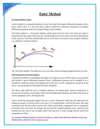
Euler's method is a numerical method to solve first order first degree differential equation with a given initial value. It is the most basic explicit method for numerical integration of ordinary differential equations and is the simplest Runge–Kutta method. The Euler method is a first-order method, which means that the local error (error per step) is proportional to the square of the step size, and the global error (error at a given time) is proportional to the step size. The Euler method often serves as the basis to construct more complex methods, e.g., predictor–corrector method

1. Dr. Umakant Bhaskar Gohatre, Assistant Professor, SIGCE, Navi Mumbai, Mumbai University,
Maharashtra, India (This file for study purpose)
1
Euler Method
Dr. Umakant Bhaskar Gohatre
Euler's method is a numerical method to solve first order first degree differential equation with a
given initial value. It is the most basic explicit method for numerical integration of ordinary
differential equations and is the simplest Runge–Kutta method.
The Euler method is a first-order method, which means that the local error (error per step) is
proportional to the square of the step size, and the global error (error at a given time) is proportional
to the step size. The Euler method often serves as the basis to construct more complex methods,
e.g., predictor–corrector method
Fig. The Euler method. The unknown curve is in blue, and its polygonal approximation is in red.
Informal geometrical description
Consider the problem of calculating the shape of an unknown curve which starts at a given point
and satisfies a given differential equation. Here, a differential equation can be thought of as a
formula by which the slope of the tangent line to the curve can be computed at any point on the
curve, once the position of that point has been calculated.
The idea is that while the curve is initially unknown, its starting point, which we denote by is
known (see the picture on top right). Then, from the differential equation, the slope to the curve at
can be computed, and so, the tangent line.
Take a small step along that tangent line up to a point Along this small step, the slope does not
change too much, so will be close to the curve. If we pretend that is still on the curve, the same
reasoning as for the point above can be used. After several steps, a polygonal curve is computed.
In general, this curve does not diverge too far from the original unknown curve, and the error
between the two curves can be made small if the step size is small enough and the interval of
computation is finite

2. Dr. Umakant Bhaskar Gohatre, Assistant Professor, SIGCE, Navi Mumbai, Mumbai University,
Maharashtra, India (This file for study purpose)
2
𝑦′(𝑡) = 𝑓(𝑡, 𝑦(𝑡)), 𝑦(𝑡0) = 𝑦0.
Choose a value for the size of every step and set 𝑡𝑛 = 𝑡0 + 𝑛ℎ. Now, one step of the Euler method
from 𝑡𝑛+1 = 𝑡𝑛 + ℎ to is 𝑦𝑛+1 = 𝑦𝑛 + ℎ𝑓(𝑡𝑛, 𝑦𝑛).
The value of 𝑦𝑛 is an approximation of the solution to the ODE at time 𝑦𝑛 ≈ 𝑦(𝑡𝑛) : The Euler
method is explicit, i.e. the solution 𝑦𝑛+1 is an explicit function of 𝑦𝑖for 𝑖 ≤ 𝑛
While the Euler method integrates a first-order ODE, any ODE of order N can be represented as a
first-order ODE: to treat the equation
𝑦(𝑁)
(𝑡) = 𝑓(𝑡, 𝑦(𝑡), 𝑦′
(𝑡), … , 𝑦(𝑁−1)
(𝑡))
we introduce auxiliary variables 𝑧1(𝑡) = 𝑦(𝑡), 𝑧2(𝑡) = 𝑦′
(𝑡), … , 𝑧𝑁(𝑡) = 𝑦(𝑁−1)
(𝑡) and obtain
the equivalent equation
𝐳′
(𝑡) = (
𝑧1
′
(𝑡)
⋮
𝑧𝑁−1
′
(𝑡)
𝑧𝑁
′
(𝑡)
) = (
𝑦′
(𝑡)
⋮
𝑦(𝑁−1)
(𝑡)
𝑦(𝑁)
(𝑡)
) = (
𝑧2(𝑡)
⋮
𝑧𝑁(𝑡)
𝑓(𝑡, 𝑧1(𝑡), … , 𝑧𝑁(𝑡))
)
This is a first-order system in the variable 𝐳(𝑡) and can be handled by Euler's method or, in fact,
by any other scheme for first-order systems.
Derivation
The Euler method can be derived in a number of ways. Firstly, there is the geometrical
description above.
Another possibility is to consider the Taylor expansion of the function 𝑦 around 𝑡0:
𝑦(𝑡0 + ℎ) = 𝑦(𝑡0) + ℎ𝑦′
(𝑡0) +
1
2
ℎ2
𝑦″
(𝑡0) + 𝑂(ℎ3
).
The differential equation states that 𝑦′
= 𝑓(𝑡, 𝑦) If this is substituted in the Taylor expansion and
the quadratic and higher-order terms are ignored, the Euler method arises.
The Taylor expansion is used below to analyze the error committed by the Euler method, and it
can be extended to produce Runge–Kutta methods.
A closely related derivation is to substitute the forward finite difference formula for the
derivative

3. Dr. Umakant Bhaskar Gohatre, Assistant Professor, SIGCE, Navi Mumbai, Mumbai University,
Maharashtra, India (This file for study purpose)
3
𝑦′(𝑡0) ≈
𝑦(𝑡0 + ℎ) − 𝑦(𝑡0)
ℎ
in the differential equation 𝑦′
= 𝑓(𝑡, 𝑦) Again, this yields the Euler method. A similar
computation leads to the midpoint method and the backward Euler method.
Finally, one can integrate the differential equation from 𝑡0 + ℎ and apply the fundamental
theorem of calculus to get
𝑦(𝑡0 + ℎ) − 𝑦(𝑡0) = ∫
𝑡0+ℎ
𝑡0
𝑓(𝑡, 𝑦(𝑡))d𝑡.
Now approximate the integral by the left-hand rectangle method
∫
𝑡0+ℎ
𝑡0
𝑓(𝑡, 𝑦(𝑡))d𝑡 ≈ ℎ𝑓(𝑡0, 𝑦(𝑡0)).
Local truncation error
The local truncation error of the Euler method is the error made in a single step
𝑦1 = 𝑦0 + ℎ𝑓(𝑡0, 𝑦0).
For the exact solution, we use the Taylor expansion mentioned in the section Derivation above
𝑦(𝑡0 + ℎ) = 𝑦(𝑡0) + ℎ𝑦′(𝑡0) +
1
2
ℎ2
𝑦″(𝑡0) + 𝑂(ℎ3).
The local truncation error (LTE) introduced by the Euler method is given by the difference
between these equations
LTE = 𝑦(𝑡0 + ℎ) − 𝑦1 =
1
2
ℎ2
𝑦″(𝑡0) + 𝑂(ℎ3).
A slightly different formulation for the local truncation error can be obtained by using the
Lagrange form for the remainder term in Taylor's theorem
If 𝑦 has a continuous second derivative, then there exists a 𝜉 ∈ [𝑡0, 𝑡0 + ℎ] such that

4. Dr. Umakant Bhaskar Gohatre, Assistant Professor, SIGCE, Navi Mumbai, Mumbai University,
Maharashtra, India (This file for study purpose)
4
LTE = 𝑦(𝑡0 + ℎ) − 𝑦1 =
1
2
ℎ2
𝑦″
(𝜉).
In the above expressions for the error, the second derivative of the unknown exact solution can
be replaced by an expression involving the right-hand side of the differential equation. Indeed, it
follows from the equation 𝑦′
= 𝑓(𝑡, 𝑦)
𝑦″(𝑡0) =
∂𝑓
∂𝑡
(𝑡0, 𝑦(𝑡0)) +
∂𝑓
∂𝑦
(𝑡0, 𝑦(𝑡0))𝑓(𝑡0, 𝑦(𝑡0)).
Global truncation error
The global truncation error is the error at a fixed time t , after however many steps the methods
needs to take to reach that time from the initial time. The global truncation error is the
cumulative effect of the local truncation errors committed in each step
|GTE| ≤
ℎ𝑀
2𝐿
(𝑒𝐿(𝑡−𝑡0)
− 1)
where M is an upper bound on the second derivative of y on the given interval and L is the
Lipschitz constant of f .
Numerical stability
If the Euler method is applied to the linear equation 𝑦′
= 𝑘𝑦 then the numerical solution is
unstable if the product ℎ𝑘 is outside the region
{ 𝑧 ∈ 𝐂 ∣ |𝑧 + 1| ≤ 1 },

5. Dr. Umakant Bhaskar Gohatre, Assistant Professor, SIGCE, Navi Mumbai, Mumbai University,
Maharashtra, India (This file for study purpose)
5
Fig. The black curve shows the exact solution.
Modifications and extensions
The backward Euler method
𝑦𝑛+1 = 𝑦𝑛 + ℎ𝑓(𝑡𝑛+1, 𝑦𝑛+1)
The midpoint method
𝑦𝑛+1 = 𝑦𝑛 + ℎ𝑓 (𝑡𝑛 +
1
2
ℎ, 𝑦𝑛 +
1
2
ℎ𝑓(𝑡𝑛, 𝑦𝑛))
The two-step Adams–Bashforth method
𝑦𝑛+1 = 𝑦𝑛 +
3
2
ℎ𝑓(𝑡𝑛, 𝑦𝑛) −
1
2
ℎ𝑓(𝑡𝑛−1, 𝑦𝑛−1).