SlideShare uma empresa Scribd logo
1 de 72
Baixar para ler offline
6. Aerodynamics of 3D Lifting Surfaces 
through Vortex Lattice Methods 
6.1 An Introduction 
There is a method that is similar to panel methods but very easy to use and capable of providing 
remarkable insight into wing aerodynamics and component interaction. It is the vortex lattice 
method (vlm), and was among the earliest methods utilizing computers to actually assist 
aerodynamicists in estimating aircraft aerodynamics. Vortex lattice methods are based on 
solutions to Laplace’s Equation, and are subject to the same basic theoretical restrictions that 
apply to panel methods. 
As a comparison, vortex lattice methods are: 
Similar to Panel methods: 
• singularities are placed on a surface 
• the non-penetration condition is satisfied at a number of control points 
• a system of linear algebraic equations is solved to determine singularity strengths 
Different from Panel methods: 
• Oriented toward lifting effects, and classical formulations ignore thickness 
• Boundary conditions (BCs) are applied on a mean surface, not the actual surface 
(not an exact solution of Laplace’s equation over a body, but embodies some 
additional approximations, i.e., together with the first item, we find DCp, 
not Cpupper and Cplower) 
• Singularities are not distributed over the entire surface 
• Oriented toward combinations of thin lifting surfaces 
(recall Panel methods had no limitations on thickness). 
Vortex lattice methods were first formulated in the late ’30s, and the method was first called 
“Vortex Lattice” in 1943 by Faulkner. The concept is extremely simple, but because of its purely 
numerical approach (i.e., no answers are available at all without finding the numerical solution of 
a matrix too large for routine hand calculation) practical applications awaited sufficient 
development of computers—the early ’60s saw widespread adoption of the method. A workshop 
was devoted to these methods at NASA in the mid ’70s.1 A nearly universal standard for vortex 
lattice predictions was established by a code developed at NASA Langley (the various versions 
were available prior to the report dates): 
Margason & Lamar2 1st Langley report NASA TN D-6142 1971 
Lamar & Gloss3 2nd " " NASA TN D-7921 1975 
Lamar & Herbert4,5 3rd " " NASA TM 83303 1982 
3/11/98 6 - 1
6 - 2 Applied Computational Aerodynamics 
Each new version had considerably more capability than the previous version. The “final” 
development in this series is designated VLM4.997. The original codes could handle two lifting 
surfaces, while VLM4.997 could handle four. Many, many other people have written vortex 
lattice method codes, some possibly even better than the code described in the NASA reports. 
But the NASA code’s general availability, versatility, and reliability resulted in its becoming a 
de-facto standard. 
Some of the most noteworthy variations on the basic method have been developed by Lan6 
(Quasi-Vortex Lattice Method), Hough7, DeJarnette8 and Frink9. Mook10 and co-workers at 
Virginia Tech have developed vortex lattice class methods that treat flowfields that contain 
leading edge vortex type separation (see Section 6.12) and also handle general unsteady motions. 
The recent book by Katz and Plotkin11 contains another variation. At Virginia Tech, Jacob Kay 
wrote a code using the method of Katz and Plotkin to estimate stability derivatives, which is 
available from the department web page.12 
To understand the method, a number of basic concepts must be reviewed. Then we describe 
one implementation of the vlm method, and use it to obtain insights into wing and wing-canard 
aerodynamics. Naturally, the method is based on the idea of a vortex singularity as the solution 
of Laplace’s equation. A good description of the basic theory for vortices in inviscid flow and 
thin wing analysis is contained in Karamcheti,13 pp. 494-496, 499-500, and 518-534. A good 
description of the vortex lattice method is given by Bertin and Smith.14 After the discussion of 
wing and wing-canard aerodynamics, an example of a vortex lattice method used in a design 
mode is presented, where the camber line required to produce a specified loading is found. The 
chapter concludes with a few examples of the extension of vortex lattice methods to treat 
situations with more complicated flowfields than the method was originally intended to treat. 
6.2 Boundary conditions on the mean surface and the pressure relation 
An important difference between vortex lattice methods and panel methods is the method in 
which the boundary conditions are handled. Typically, the vortex lattice method uses an 
approximate boundary condition treatment. This boundary condition can also be used in other 
circumstances to good advantage. This is a good “trick” applied aerodynamicists should know 
and understand. In general, this approach results in the so-called “thin airfoil boundary 
condition,” and arises by linearizing and transferring the boundary condition from the actual 
surface to a flat mean “reference” surface, which is typically a constant coordinate surface. 
Consistent with the boundary condition simplification, a simplified relation between the pressure 
and velocity is also possible. The simplification in the boundary condition and pressure-velocity 
relation provides a basis for treating the problem as a superposition of the lift and thickness 
contributions to the aerodynamic results. Karamcheti13 provides an excellent discussion of this 
approach. 
3/11/98
Aerodynamics of 3D Lifting Surfaces 6 - 3 
To understand the thin airfoil theory boundary condition treatment, we provide an example in 
two dimensions. Recall (from Eqn. 2-54) that the exact surface boundary condition for steady 
inviscid flow is: 
3/11/98 
V×n = 0 (6-1) 
on F(x, y) = 0 = y − f (x) . The unit normal vector is n = ÑF(x, y) / ÑF(x, y) and the velocity 
field is defined using the notation defined in Fig. 6-1. 
V 
V cos 
a V sin 
a 
a 
¥ 
¥ 
¥ 
y 
x 
Figure 6-1. Basic coordinate system for boundary condition analysis. 
Define the velocity components of V as: 
V = V¥ + q(x,y) 
   
1  2  3  
a disturbance velocity 
(6-2) 
where q is a disturbance velocity with components u and v. If we assume irrotational flow, then 
these components are described in terms of a scalar potential function, u = Ñfx and v = Ñfy. The 
total velocity V then becomes in terms of velocity components: 
uTOT = V¥ cosa + u(x,y) 
vTOT = V¥ sina + v(x, y) 
(6-3) 
and we can write out the boundary condition as: 
V×n = (uTOTi + vTOTj) × 
¶F 
¶x 
i + 
¶F 
¶ y 
j 
æ  
è  
ç  
ö  
ø  
÷ = 0 (6-4) 
or 
[V¥ cosa + u(x, y)]¶F 
¶x 
+[V¥ sina + v(x, y)] ¶F 
¶y 
= 0 (6-5) 
on F(x,y) = 0, and recalling the relationship between F and f given below Eqn. (6-1):
6 - 4 Applied Computational Aerodynamics 
3/11/98 
¶F 
¶x 
= ¶ 
¶ x 
{y − f (x)} = − df (x) 
dx 
¶F 
¶y 
= ¶ 
¶ y 
{y − f (x)} = 1 
. (6-7) 
Substituting for F in Eq.(6-5) we have: 
(V¥ cosa + u) − df 
dx 
æ  
è  
ç  ö  
÷ + (V¥ sina + v) = 0 (6-8) 
ø  
which, solving for v, is: 
v =(V¥ cosa + u) df 
dx 
− V¥ sina (6-9) 
on y = f(x). Note that v is defined in terms of the unknown u. Thus Eq. (6-9) is a nonlinear 
boundary condition and further analysis is needed to obtain a useful relation.* 
6.2.1 Linearized form of the boundary condition 
The relation given above by Eq.(6-9) is exact. It has been derived as the starting point for 
the derivation of useful relations when the body (which is assumed to be a thin surface at a small 
angle of attack) induces disturbances to the freestream velocity that are small in comparison to 
the freestream velocity. Thus we assume: u << V¥, v << V¥, and ¶F/¶x < ¶F/¶y. Note that this 
introduces a bias in the coordinate system to simplify the analysis, a typical consequence of 
introducing simplifying assumptions. Consistent with this assumption, the components of the 
freestream velocity are: 
V¥ cosa » V¥ 
V¥sina » V¥a 
(6-10) 
and the expression for v in Eq.(6-9) becomes: 
v = (V¥ + u) df 
dx 
−V¥a . (6-11) 
Dividing by V¥, 
v 
V¥ 
= 1+ u 
V¥ 
æ  
è  
ç  
ö  
ø  
df 
dx 
÷  
− a (6-12) 
the linearized boundary condition is obtained by neglecting u/V¥ compared with unity 
(consistent with the previous approximations). With this assumption, the linearized boundary 
condition becomes: 
v 
V¥ 
= df 
dx 
− a on y = f (x) . (6-13) 
* Observe that even when the flowfield model is defined by a linear partial differential equation, an 
assumption which we have not yet made, the boundary condition can make the problem nonlinear.
Aerodynamics of 3D Lifting Surfaces 6 - 5 
This form of the boundary condition is not valid if the flow disturbance is large compared to 
the freestream velocity {for aerodynamically streamlined shapes this is usually valid everywhere 
except at the leading edge of the airfoil, where a stagnation point exists (u = -V¥) and the slope 
is infinite (df/dx = ¥ )}. In practice, a local violation of this assumption leads to a local error. 
Thus, if the details of the flow at the leading edge are not important to the analysis, which 
surprisingly is often the case, the linearized boundary condition can be used. 
6.2.2 Transfer of the boundary condition 
Although Eqn. (6-13) is linear, it’s hard to apply because it is not applied on a coordinate 
line.* We now use a further approximation of this relation to get the useful form of the linearized 
boundary condition. Using a Taylor series expansion of the v component of velocity about the 
coordinate axis we obtain the v velocity on the surface: 
3/11/98 
v{x, y = f(x)} = v(x,0) + f (x) 
¶v 
¶y y=0 
+... . (6-14) 
For the thin surfaces under consideration, f(x) is small, and because the disturbances are assumed 
small, ¶v/¶y is also small. For example, assume that v and ¶v/¶y are the same size, equal to 0.1, 
and df/dy is also about 0.1. The relation between v on the airfoil surface and the axis is: 
{ . (6-15) 
v{x, y = f(x)} = (.1) +(.1)(.1) = .1 + .01 
   
neglect 
Neglecting the second term, we assume: 
v{x, f (x)} » v(x, 0). (6-16) 
We now apply both the upper and lower surface boundary conditions on the axis y = 0, and 
distinguish between the upper and lower surface shapes by using: 
f = fu on the upper surface 
f = fl on the lower surface 
. (6-17) 
Using Eq. (6-17), we write the upper and lower surface boundary conditions as: 
v(x,0+ ) 
V¥ 
up 
= dfu 
dx 
− a, 
v(x,0− ) 
V¥ 
low 
= dfl 
dx 
− a . (6-18) 
* The simplification introduced by applying boundary conditions on constant coordinate surfaces justifies 
the use of rather elaborate tranformations, which will be dicussed in more detail in Chap. 9, Geometry and 
Aerodynamics.
6 - 6 Applied Computational Aerodynamics 
These are the linearized and transferred boundary conditions. Frequently, these boundary 
conditions result in a surprisingly good approximation to the flowfield, even in transonic and 
supersonic flow. 
6.2.3 Decomposition of boundary conditions to camber/thickness/alpha 
Further simplification and insight can be gained by considering the airfoils in terms of the 
combination of thickness and camber, a natural point of view. We thus write the upper and lower 
surface shapes in terms of camber, fc, and thickness, ft, as: 
3/11/98 
fu = fc + ft 
fl = fc − ft 
(6-19) 
and the general problem is then divided into the sum of three parts as shown in Fig. 6-2. 
General 
airfoil 
at a 
Thickness 
at a = 0° 
Camber 
at a = 0° 
Flat plate 
at a 
= + + 
Figure 6-2. Decomposition of a general shape at incidence. 
The decomposition of the problem is somewhat arbitrary. Camber could also be considered 
to include angle of attack effects using the boundary condition relations given above, the sign is 
the same for both the upper and lower surface. The aerodynamicist must keep track of details for 
a particular problem. To proceed further, we make use of the basic vortex lattice method 
assumption: the flowfield is governed by a linear partial differential equation (Laplace’s 
equation). Superposition allows us to solve the problem in pieces and add up the contributions 
from the various parts of the problem. This results in the final form of the thin airfoil theory 
boundary conditions: 
v(x,0+ ) 
V¥ 
up 
= dfc 
dx 
+ dft 
dx 
−a 
v(x,0− ) 
V¥ 
low 
= dfc 
dx 
− dft 
dx 
−a 
. (6-20) 
The problem can be solved for the various contributions and the contributions are added together 
to obtain the complete solution. If thickness is neglected the boundary conditions are the same 
for the upper and lower surface.
Aerodynamics of 3D Lifting Surfaces 6 - 7 
6.2.4 Thin airfoil theory pressure relation 
Consistent with the linearization of the boundary conditions, a useful relation between the 
pressure and velocity can also be obtained. For incompressible flows, the exact relation between 
pressure and velocity is: 
3/11/98 
æ  
è  
Cp =1 − V 
ç  
V¥ 
2 
ö  
÷  
ø  
(6-21) 
and we expand the velocity considering disturbances to the freestream velocity using the 
approximations discussed above: 
V2 = (V¥ cosa + u)2 +(V¥ sin a + v)2 
V¥ V¥a 
. 
Expanding: 
2 + 2V¥u + u2 + (V¥a)2 + 2V¥av + v2 (6-22) 
V 2 = V¥ 
2 we get: 
and dividing by V¥ 
V 2 
V¥ 
2 =1 + 2 
u 
V¥ 
+ u2 
V¥ 
2 + a 2 + 2a v 
V¥ 
+ v2 
V¥ 
2 . (6-23) 
Substituting into the Cp relation, Eqn. (6-21), we get: 
CP = 1− 1 + 2 
u 
V¥ 
+ u2 
V¥ 
2 + a 2 + 2a v 
V¥ 
+ v2 
V¥ 2 
æ  
è  
ç  
ö  
÷  
ø  
= 1− 1− 2 
u 
V¥ 
− u2 
V¥ 
2 − a 2 − 2a v 
V¥ 
− v2 
V¥ 2 
(6-24) 
and if a, u/V¥ and v/V¥ are << 1, then the last four terms can be neglected in comparison with 
the third term. The final result is: 
Cp =− 2 
u 
V¥ 
. (6-25) 
This is the linearized or “thin airfoil theory pressure formula”. From experience gained 
comparing various computational results, I’ve found that this formula is a slightly more severe 
restriction on the accuracy of the solution than the linearized boundary condition. Equation (6- 
25) shows that under the small disturbance approximation, the pressure is a linear function of u, 
and we can add the Cp contribution from thickness, camber, and angle of attack by 
superposition. A similar derivation can be used to show that Eq. (6-25) is also valid for 
compressible flow up to moderate supersonic speeds.
6 - 8 Applied Computational Aerodynamics 
6.2.5 Delta Cp due to camber/alpha (thickness cancels) 
Next, we make use of the result in Eq. (6-25) to obtain a formula for the load distribution on 
the wing: 
3/11/98 
DCp = CpLOWER −CpUPPER . (6-26) 
Using superposition, the pressures can be obtained as the contributions from wing thickness, 
camber, and angle of attack effects: 
CpLOWER =CpTHICKNESS +CpCAMBER + CpANGLE OF ATTACK 
CpUPPER =CpTHICKNESS −CpCAMBER −CpANGLE OF ATTACK 
(6-27) 
so that: 
DCp = CpTHICKNESS +CpCAMBER +CpANGLE OF ATTACK ( ) 
− CpTHICKNESS − CpCAMBER −CpANGLE OF ATTACK ( ) 
= 2 CpCAMBER +CpANGLE OF ATTACK ( ) 
. (6-28) 
Equation (6-28) demonstrates that for cases where the linearized pressure coefficient relation is 
valid, thickness does not contribute to lift to 1st order in the velocity disturbance! 
The importance of this analysis is that we have shown: 
1. how the lifting effects can be obtained without considering thickness, and 
2. that the cambered surface boundary conditions can be applied on a flat coordinate 
surface, resulting in an easy to apply boundary condition. 
The principles demonstrated here for transfer and linearization of boundary conditions can be 
applied in a variety of situations other than the application in vortex lattice methods. Often this 
idea can be used to handle complicated geometries that can’t easily be treated exactly. 
The analysis here produced an entirely consistent problem formulation. This includes the 
linearization of the boundary condition, the transfer of the boundary condition, and the 
approximation between velocity and pressure. All approximations are consistent with each other. 
Improving one of these approximations without improving them all in a consistent manner may 
actually lead to worse results. Sometimes you can make agreement with data better, sometimes it 
may get worse. You have to be careful when trying to improve theory on an ad hoc basis.
Aerodynamics of 3D Lifting Surfaces 6 - 9 
6.3 Vortex Theorems 
In using vortex singularities to model lifting surfaces, we need to review some properties of 
vortices. The key properties are defined by the so-called vortex theorems. These theorems are 
associated with the names of Kelvin and Helmholtz, and are proven in Karamcheti.13 Three 
important results are: 
3/11/98 
1. Along a vortex line (tube) the circulation, G, is constant. 
2. A vortex filament (or line) cannot begin or end abruptly in a fluid. The vortex line 
must i) be closed, ii) extend to infinity, or iii) end at a solid boundary. 
Furthermore, the circulation, G, about any section is the vortex strength. 
3. An initially irrotational, inviscid flow will remain irrotational. 
Related to these theorems we state an important result: 
• A sheet of vortices can support a jump in tangential velocity [i.e. a force], 
while the normal velocity is continuous. This means you can use a vortex sheet 
to represent a lifting surface. 
6.4 Biot-Savart Law 
We know that a two-dimensional vortex singularity satisfies Laplace’s equation (i.e. a point 
vortex): 
V = 
G 
2p r 
eq (6-29) 
where Vq is the irrotational vortex flow illustrated in Fig. 6-3. 
Vq 
Vortex normal 
to page 
r 
V 
q 
1/r 
. 
a) streamlines b) velocity distribution 
Figure 6-3. The point vortex. 
What is the extension of the point vortex idea to the case of a general three-dimensional 
vortex filament? Consider the flowfield induced by the vortex filament shown in Fig. 6-4, which 
defines the nomenclature.
6 - 10 Applied Computational Aerodynamics 
3/11/98 
G 
dl 
q 
p 
rpq 
vortex 
filament 
Figure 6-4. General three-dimensional vortex filament. 
The mathematical description of the flow induced by this filament is given by the Biot- 
Savart law (see Karamcheti,13 pages 518-534). It states that the increment in velocity dV at a 
point p due to a segment of a vortex filament dl at q is: 
dVp = 
G 
4p 
× 
dl × rpq 
rpq 
3 . (6-30) 
To obtain the velocity induced by the entire length of the filament, integrate over the length 
of the vortex filament (or line) recalling that G is constant. We obtain: 
r  
V p = 
   
G 
4p 
r  
l × r  
d 
r pq 
r  
r pq 
3 
ó  
õ  
ô  
ô  . (6-31) 
To illustrate the evaluation of this integral we give the details for several important 
examples. The vector cross product definition is reviewed in the sidebar below. Reviewing the 
cross product properties we see that the velocity direction dVp induced by the segment of the 
vortex filament dl is perpendicular to the plane defined by dl and rpq, and its magnitude is 
computed from Eq. (6-31). 
Case #1: the infinitely long straight vortex. 
In the first illustration of the computation of the induced velocity using the Biot-Savart Law, we 
consider the case of an infinitely long straight vortex filament. The notation is given in Fig. 6-5.
Aerodynamics of 3D Lifting Surfaces 6 - 11 
A review: the meaning of the cross product. What does a x b mean? Consider the following 
sketch: 
Here, the vectors a and b form a plane, and the result of the cross product operation is a vector c, 
where c is perpendicular to the plane defined by a and b. The value is given by: 
and e is perpendicular to the plane of a and b. One consequence of this is that if a and b are 
parallel, then a x b = 0. 
Also: a × b = area of the parallelogram 
and 
3/11/98 
+ ¥ 
p 
c = a × b = a b sinq e 
dl 
G 
q 
h 
q 
rpq 
c 
- ¥ 
. 
a 
b 
q 
Figure 6-5. The infinitely long straight vortex. 
a × b = 
i j k 
Ax Ay Az 
Bx By Bz 
= (AyBz − AzBy )i −(AxBz − AzBx)j + (Ax By − AyBx)k
6 - 12 Applied Computational Aerodynamics 
Now consider the numerator in Eq. (6-30) given above using the definition of the cross 
product: 
3/11/98 
dl × rpq = dl rpq sinq 
V 
V 
(6-32) 
so that the entire expression becomes 
dVp = 
G 
4p 
× 
dl rpq sinq 
3 
rpq 
V 
V 
= G 
4p 
V 
V 
sinq dl 
rpq 
2 
. (6-33) 
Next, simplify the above expressions so they can be readily evaluated. Use the nomenclature 
shown in Fig. 6-6. 
p 
q 
l1 l 
h 
rpq 
q 
Figure 6-6. Relations for the solution of the Biot-Savart Law. 
Using the notation in Fig. 6-6 to find the relations for rpq and dl. First we see that: 
h = rpq sinq (6-34) 
or rpq = h 
sinq 
(6-35) 
and l1 − l = h 
tanq 
= hcotq . (6-36) 
Next look at changes with q. Start by taking the differential of Eq. (6-36): 
which is 
d(l1 − l) = d 
æ  
è  
ç  ö  
h 
tanq 
÷ = d(hcotq) 
ø  
−dl = h d(cot q) 
− dl 
dq 
= h 
d 
dq 
(cotq) = −hcosec2q 
(6-37) 
and we can now write dl in terms of dq : 
dl = hcosec2q dq (6-38)
Aerodynamics of 3D Lifting Surfaces 6 - 13 
so that the Biot-Savart Law gives: 
3/11/98 
dVp = G 
4p 
V 
V 
sinq dl 
rpq 
2 
= 
G 
4p 
V 
V 
sinq hcosec2q dq 
æ  
è  
2 
ç  ö  
h 
sinq 
÷  
ø  
= 
G 
4p 
sinq 
h 
dq (direction understood) 
. (6-39) 
Thus we integrate: 
Vp = 
G 
4p 
sinq 
h 
ò dq = 
G 
4p h 
q=p 
ò (6-40) 
sinq dq 
q =0 
where here the limits of integration would change if you were to consider a finite straight length. 
Carrying out the integration: 
Vp = G 
[−cosq ]q =0 
4p h 
q =p 
= 
G 
4p h 
[−(−1) − (−1)] 
and: 
Vp = 
G 
2p h 
(6-41) 
which agrees with the two dimensional result. 
Although a vortex cannot end in a fluid, we can construct expressions for infinitely long 
vortex lines made up of a series of connected straight line segments by combining expressions 
developed using the method illustrated here. To do this we simply change the limits of 
integration. Two cases are extremely useful for construction of vortex systems, and the formulas 
are given here without derivation. 
Case #2: the semi-infinite vortex. 
This expression is useful for modeling the vortex extending from the wing to downstream 
infinity. 
+ ¥ 
p 
dl 
G 
q 
q0 
h 
Vp = 
G 
4ph 
(1 + cosq0 )e (6-42) 
Figure 6-7. The semi-infinite vortex.
6 - 14 Applied Computational Aerodynamics 
Case #3: the finite vortex. 
This expression can be used to model the vortex on a wing, and can be joined with two 
semi-infinite vortices to form a vortex of infinite length, satisfying the vortex theorems. 
3/11/98 
p 
dl 
G 
q 
q1 
h 
q2 
Vp = 
G 
4ph 
(cosq1 − cosq2 )e (6-43) 
Figure 6-8. The finite vortex. 
Systems of vortices can be built up using Eqns. (6-42) and (6-43) and the vortex theorems. 
The algebra can become tedious, but there are no conceptual difficulties. 
6.5 The Horseshoe Vortex 
There is a specific form of vortex used in the traditional vortex lattice method. We now use 
the expressions developed from the Biot-Savart Law to create a “horseshoe vortex”, which 
extends from downstream infinity to a point in the field “A”, then from point “A” to point “B,” 
and another vortex from point “B” downstream to infinity. The velocity induced by this vortex is 
the sum of the three parts. The basic formulas were presented in the previous section. Here we 
extend the analysis of the previous section, following the derivation and notation of Bertin and 
Smith.14 In particular, the directions of the induced flow are made more precise. Our goal is to 
obtain the expression for the velocity field at a general point in space (x,y,z) due to the specified 
horseshoe vortex. 
To create a horseshoe vortex we will use three straight line vortices: one finite length vortex 
and two semi-infinite vortices. This is illustrated in Fig. 6-9. To start our analysis, we rewrite the 
Biot-Savart Law in the Bertin and Smith notation,14 which is given in Fig. 6-10.
Aerodynamics of 3D Lifting Surfaces 6 - 15 
3/11/98 
¥ 
¥ 
A 
B 
G 
G 
G 
Figure 6-9. The horseshoe vortex. 
A 
B 
C 
r1 
r 
r2 
dl rp 
q2 
q 
q 1 ro = AB 
r1 = AC 
r2 = BC 
Figure 6-10. Nomenclature for induced velocity calculation. 
The next step is to relate the angles to the vector definitions. The definition of the dot product 
is used: 
A×B= A B cosq (6-44) 
so that: 
cosq1 = 
r0 ×r1 
r0 r1 
cosq2 = 
r0 × r2 
r0 r2 
. (6-45) 
Next, we put these relations into the formula for the finite length vortex segment formula for the 
induced velocity field given above in Eq. (6-43). 
Vp = 
G 
4p rp 
(cosq1 − cosq2)e (6-46) 
so that, substituting using the definition in Eq. (6-44), we get 
Vp = 
G 
4p 
r0 
r1 × r2 
r0 × r1 
r0 r1 
− 
r0 × r2 
r0 r2 
æ  
è  
ç  
ö  
÷  
ø  
r1 × r2 
r1 × r2 
. (6-47)
6 - 16 Applied Computational Aerodynamics 
Bertin and Smith14 use the relation: 
rp = 
r1 × r2 
r0 
rp = 
r1 × r2 
r0 
and we need to demonstrate that this is true. Consider the parallelogram ABCD shown in the 
sketch: 
A 
D C 
rp 
B 
r 
1 
r 
2 
r 
0 
by definition: r1 × r2 = Ap , is the area of the parallelogram. 
Similarly, the area of ABC is: 
AABC = 1 
2 
bh 
= 1 
2 
ro rp 
The total area of the parallelogram can be found from both formulas, and by equating these two 
areas we obtain the expression we are trying to get: 
2AABC = Ap 
ro rp = r1 × r2 
which can be rewritten to obtain the expression given by Bertin and Smith:14 
rp = 
r1 × r2 
r0 
Collecting terms and making use of the vector identity provided in the sidebar, we obtain the 
Bertin and Smith statement of the Biot-Savart Law for a finite length vortex segment: 
3/11/98 
Vp = 
G 
4p 
r1 × r2 
r1 × r2 
2 r0 × 
r1 
r1 
− 
r2 
r2 
æ  
è  
ç  
ö  
÷  
ø  
é  
ê  
ë  
ù  
û  
ú . (6-48) 
For a single infinite length horseshoe vortex we will use three segments, each using the 
formula given above. The nomenclature is given in the sketch below. The primary points are the
Aerodynamics of 3D Lifting Surfaces 6 - 17 
connecting points A and B. Between A and B we use a finite length vortex which is considered a 
“bound” vortex, and from A to infinity and B to infinity we define “trailing” vortices that are 
parallel to the x-axis. 
The general expression for the velocity at a point x, y, z due to a horseshoe vortex at (x1n, 
y1n, z1n), (x2n,y2n, z2n) with trailing vortices parallel to the x-axis is (from Bertin and Smith14): 
3/11/98 
V = VAB +VA¥ +VB¥ (6-49) 
where the total velocity is the sum of the contributions from the three separate straight line 
vortex segments making up the horseshoe vortex, as shown in Fig. 6-11. 
¥ 
¥ 
A 
B 
G 
G 
G 
n 
n 
n 
x 
z 
y 
Figure 6-11. Definitions for notation used in induced velocity expressions. 
The corner points of the vortex, A and B , are arbitrary, and are given by: 
A = A(x1n, y1n, z1n) 
B = B(x2n, y2n,z2n) 
. (6-50) 
We now write the expression for the velocity field at a general point in space (x,y,z) due to 
the horseshoe vortex system. At C(x,y,z) find the induced velocity due to each vortex segment. 
Start with AB, and use Fig. 6-12. 
Now we define the vectors as:
6 - 18 Applied Computational Aerodynamics 
3/11/98 
r0 = (x2n − x1n)i + (y2n − y1n)j + (z2n − z1n)k 
r1 = ( x − x1n )i + ( y − y1n)j + (z − z1n )k 
r0 = (x − x2n)i + (y − y2n)j + (z − z2n)k 
(6-51) 
A 
B 
C(x,y,z) 
r 
r 
r 
0 
1 
2 
Figure 6-12. Velocity induced at Point C due to the vortex between A and B. 
and we simply substitute into: 
VC = 
   
G 
4p 
r1 × r2 
r1 × r2 
2 
14  4 4 2  4  4  4 3    
14 2  4 3    
Y 
r0 × 
r1 
r1 
− r0 × 
r2 
r2 
æ  
è  
ç  
ö  
÷  
ø  
W 
. (6-52) 
Considering the bound vortex on AB first we obtain, 
VAB = 
Gn 
4p 
æ  W 
è  
ç  ö  
÷ Y (6-53) 
ø  
where Y and W are lengthy expressions. By following the vector definitions, Eqn. (6-53) can be 
written in Cartesian coordinates. The vector Y is: 
Y = r1 × r2 
r1 × r2 
2 
= 
[(y − y1n )(z − z2n) − ( y − y2n)(z − z1n)]i 
−[( x − x1n )(z − z2n) − (x − x2n)(z − z1n )]j 
+[(x − x1n )(y − y2n) −(x − x2n)(y − y1n )]k 
ì  
í  
ïï   
ï  
ï  
î  
ü  
ý  
ïï   
ï  
ï  
. (6-54) 
þ  
[(y − y1n)(z − z2n) − (y − y2n)(z − z1n)]2 
+[( x − x1n)(z − z2n) − (x − x2n)(z − z1n)]2 
+[(x − x1n)(y − y2n ) − (x − x2n )(y − y1n)]2 
ì  
ï  
ï  
í  
ï  
ï  
î  
ü  
ï  
ï  
ý  
ï  
ï  
þ
Aerodynamics of 3D Lifting Surfaces 6 - 19 
The scalar portion of the expression, W, is: 
3/11/98 
W = ro × r1 
r1 
− ro × r2 
r2 
æ  
è  
ç  
ö  
÷  
ø  
= 
[(x2n − x1n )( x − x1n ) + (y2n − y1n )( y − y1n) + (z2n − z1n)(z − z1n)] 
(x − x1n )2 + (y − y1n)2 +(z − z1n)2 
− 
[(x2n − x1n)(x − x2n) + (y2n − y1n)(y − y2n ) + (z2n − z1n)(z − z2n)] 
( x − x2n)2 +( y − y2n )2 + (z − z2n)2 
. (6-55) 
We find the contributions of the trailing vortex legs using the same formula, but redefining 
the points 1 and 2. Then, keeping the 1 and 2 notation, define a downstream point, “3” and let x3 
go to infinity. Thus the trailing vortex legs are given by: 
VA¥ = 
Gn 
4p 
ì  
í  
(z − z1n )j +( y1n − y)k 
(z − z1n)2 +(y1n − y)[ 2] 
ï  
ïî   
ü  
ý  
ï  
ïþ   
1.0 + x − x1n 
(x − x1n)2 + (y − y1n)2 + (z − z1n )2 
é  
ê  
ê  
ë  
ù  
ú  
ú  
û  
(6-56) 
and 
VB ¥ = − 
Gn 
4p 
ì  
í  
(z − z2n )j +( y2n − y)k 
(z − z2n)2 + (y2n − y)[ 2] 
ï  
ïî   
ü  
ý  
ï  
ïþ   
1.0 + x − x2n 
(x − x2n)2 + (y − y2n)2 + (z − z2n)2 
é  
ê  
ê  
ë  
ù  
ú  
ú .(6-57) 
û  
Note that Gn is contained linearly in each expression, so that the expression given above can 
be arranged much more compactly by using (6-49) with (6-52), (6-56), and (6-57) as: 
Vm = CmnGn 
(6-58) 
and Cmn is an influence coefficient for the nth horseshoe vortex effect at the location m, 
including all three segments. 
Now that we can compute the induced velocity field of a horseshoe vortex, we need to 
decide where to place the horseshoe vortices to represent a lifting surface. 
6.6 Selection of Control Point/Vortex Location 
Since we are interested in using the horseshoe vortex defined above to represent a lifting 
surface, we need to examine exactly how this might be done. In particular: where do you locate 
the vortex, and where do you locate a control point to satisfy the surface boundary condition? 
Tradition has been to determine their locations by comparison with known results. In particular, 
we use two dimensional test cases, and then apply them directly to the three dimensional case.
6 - 20 Applied Computational Aerodynamics 
An alternate distribution based on numerical properties of quadrature formulas has been derived 
by Lan. Section 6.11 will demonstrate the use of his vortex/control point locations in the inverse 
case, where the pressure is given, and the shape of the surface is sought. 
a) Simplest Approach: A Flat Plate 
Consider representing the flow over a flat plate airfoil by a single vortex and control point. 
Comparing with the known result from thin airfoil theory we determine the spacing between the 
vortex and control point which produces a lift identical with the thin airfoil theory value. 
Consider the flat plate as sketched in Fig. 6-13. 
3/11/98 
X 
c 
G 
a b 
control point 
r 
Figure 6-13. The notation for control point and vortex location analysis. 
The velocity at the control point, cp, due to the point vortex is: 
vcp = − 
G 
2pr 
. (6-59) 
The flow tangency condition was given above as: 
vBC 
V¥ 
= dfc 
dx 
−a (6-60) 
and ignoring camber: 
vBC 
V¥ 
= −a (6-61) 
or: 
vBC = −aV¥. (6-62) 
Now, we equate vBC and vcp: 
− 
G 
2pr 
= −aV¥ (6-63) 
resulting in the expression for a:
Aerodynamics of 3D Lifting Surfaces 6 - 21 
3/11/98 
a = 
G 
2prV¥ 
. (6-64) 
To make use of this relation, recall the Kutta-Joukowsky Theorem: 
L = rV¥G (6-65) 
and the result from thin airfoil theory: 
L = 12 
   
rV¥ 2 
q¥ 
c 
Sref 
12 3    
{. (6-66) 
{ 2pa 
CL 
Equate the expressions for lift, Eqns. (6-65) and (6-66) and substitute for a using the 
expression in Eqn. (6-64) given above: 
rV¥G = 12 
rV¥ 2 
c2pa 
= 12 
rV¥ 2 
c2p 
G 
2prV¥ 
1 = 1 
2 
c 
r 
(6-67) 
and finally: 
r = c 
2 
. (6-68) 
This defines the relation between the vortex placement and the control point in order for the 
single vortex model to reproduce the theoretical lift of an airfoil predicted by thin airfoil theory. 
Since the flat plate has constant (zero) camber everywhere, this case doesn’t pin down placement 
(distance of the vortex from the leading edge) completely. Intuitively, the vortex should be 
located at the quarter-chord point since that is the location of the aerodynamic center of a thin 
flat plate airfoil. The next example is used to determine the placement of the vortex. 
b) Determine placement of the vortex using parabolic camber model. 
Rewrite the velocity at the control point due to the point vortex in a little more detail, where 
a denotes the location of the vortex, and b the location of the control point: 
vcp = − 
G 
2p(a − b) (6-69) 
and the boundary condition remains the same: 
vBC = V¥ 
æ  −a 
è  
ç  ö  
dfc 
dx 
÷ . (6-70) 
ø
6 - 22 Applied Computational Aerodynamics 
Equating the above expressions (and dividing by V¥:): 
3/11/98 
− 
G 
2p(a − b)V¥ 
æ  − a 
è  
ç  ö  
= dfc 
dx 
÷ . (6-71) 
ø  
For parabolic camber, 
æ  
è  
ç  ö  
ø  
fc(x) = 4d x 
c 
÷( c − x) (6-72) 
we have the slope, 
dfc(x) 
dx 
é  ÷  
êë   
= 4d 1− 2 
æ  
è  
ç  ö  
ø  
x 
c 
ù  
úû   (6-73) 
so that: 
− 
G 
2p(a − b)V¥ 
é  æ  
êë   
÷  
è  
= 4d 1− 2 
ç  ö  
ø  
x 
c 
ù  
úû  −a . (6-74) 
Now use the result from thin airfoil theory: 
L = 12 
rV¥ 2 
c2p(a + 2d) 
and substitute for the lift from the Kutta-Joukowsky theorem. We thus obtain an expression for 
the circulation of the vortex in terms of the angle of attack and camber: 
G = pV¥c(a + 2d ). (6-75) 
Substitute for G from (6-75) into (6-74), and satisfy the boundary condition at x = b: 
−pV¥c(a + 2d ) 
2p(b − a)V¥ 
é  æ  
êë   
÷  
è  
= 4d 1 − 2 
ç  ö  
ø  
b 
c 
ù  
úû  −a 
or: 
− 1 
2 
æ  
è  
ç  ö  
c 
b − a 
é  ÷  
êë   
÷ (a + 2d) = 4d 1− 2 
ø  
æ  
è  
ç  ö  
ø  
b 
c 
ù  
úû  −a . (6-76) 
To be true for arbitrary a, d, the coefficients must be equal: 
− 1 
2 
æ  
è  
ç  ö  
c 
b − a 
÷ = −1 
ø  
æ  
è  
ç  ö  
− c 
b − a 
÷ = 4 1 − 2 
ø  
b 
c 
é  
ëê   
ù  
úû   
(6-77) 
and we solve for a and b. The first relation can be solved for (b-a): 
(b − a) = c 
2 
(6-78) 
and we obtain the same results obtained above, validating our previous analysis ( r = c/2).
Aerodynamics of 3D Lifting Surfaces 6 - 23 
Now, rewrite the 2nd equation: 
3/11/98 
é  æ  
êë   
÷  
è  
−c = 4 1− 2 
ç  ö  
ø  
b 
c 
ù  
úû(  b − a) 
or: 
é  æ  
êë   
÷  
è  
−c = 4 1− 2 
ç  ö  
ø  
b 
c 
ù  
úû   
c 
2 
(6-79) 
and solve for b/c: 
é  æ  
êë   
÷  
è  
−1 = 2 1 − 2 
ç  ö  
ø  
b 
c 
ù  
úû   
− 1 
2 
æ  
è  
=1 − 2 
ç  ö  
ø  
b 
c 
÷  
2 
b 
c 
=1 + 1 
2 
= 3 
2 
b 
c 
= 1 
2 
3 
2 
= 3 
4 , (6-80) 
and use this to solve for a/c starting with Eqn. (6-78) : 
(b − a) = c 
2 
or: 
b 
c 
− a 
c 
= 1 
2 
(6-81) 
and: 
a 
c 
= b 
c 
− 1 
2 
= 3 
4 
− 1 
2 
. 
Finally: 
a 
c 
= 1 
4 
. (6-82) 
Thus the vortex is located at the 1/4 chord point, and the control point is located at the 3/4 
chord point. Naturally, this is known as the “1/4 - 3/4 rule.” It’s not a theoretical law, simply a 
placement that works well and has become a rule of thumb. It was discovered by Italian Pistolesi. 
Mathematical derivations of more precise vortex/control point locations are available (see Lan6), 
but the 1/4 - 3/4 rule is widely used, and has proven to be sufficiently accurate in practice.
6 - 24 Applied Computational Aerodynamics 
To examine the use of these ideas we present a two-dimensional example. The airfoil is 
divided into a number of equal size panels. Each panel has a vortex at the quarter chord point and 
the non-penetration condition is satisfied at the three-quarter chord point. We use the example to 
illustrate the accuracy of the classical thin airfoil theory formulation. In Fig. 6-14, we compare 
the results obtained for a 5% circular arc camber.* Three solutions are presented. The linear 
theory curve uses classical thin airfoil theory with results obtained satisfying the boundary 
condition on the mean surface. This is compared with numerical results for the case where the 
boundary condition is applied exactly on the camber line, and the result obtained applying the 
boundary condition using the approximate method described above. The difference between 
placing the vortex on the actual camber surface and satisfying the boundary condition on the 
actual surface, and the more approximate traditional approach of locating the vortex and control 
point on the mean surface is extremely small. 
3/11/98 
0.90 
0.80 
0.70 
0.60 
0.50 
0.40 
0.30 
0.20 
0.10 
DCp 
5% Circular arc camber line 
a = 0 ° 
40 panels 
0.0 0.2 0.4 0.6 0.8 1.0 
x/c 
DCp bc's on camber line 
DCp bc's on axis 
DCp linear theory 
Figure 6-14. Comparison in 2D of the 1/4-3/4 rule for vortex-control point locations with 
linear theory, and including a comparison between placing the vortex and 
control point on the camber line or on the axis. 
* A relatively large camber for a practical airfoil, the NACA 4412 example we used in Chapter 4 was an extreme 
case, and it has 4% camber.
Aerodynamics of 3D Lifting Surfaces 6 - 25 
6.7 The Classical Vortex Lattice Method 
There are many different vortex lattice schemes. In this section we describe the “classical” 
implementation. Knowing that vortices can represent lift from our airfoil analysis, and that one 
approach is to place the vortex and then satisfy the boundary condition using the “1/4 - 3/4 rule,” 
we proceed as follows: 
3/11/98 
1. Divide the planform up into a lattice of quadrilateral panels, and put a horseshoe 
vortex on each panel. 
2. Place the bound vortex of the horseshoe vortex on the 1/4 chord element line of 
each panel. 
3. Place the control point on the 3/4 chord point of each panel at the midpoint in the 
spanwise direction (sometimes the lateral panel centroid location is used) . 
4. Assume a flat wake in the usual classical method. 
5. Determine the strengths of each Gn required to satisfy the boundary conditions by 
solving a system of linear equations. The implementation is shown schematically 
in Fig. 6-15. 
y 
x 
X 
X 
X 
bound vortices 
X 
X 
control points 
X 
X 
X 
X 
Trailing vortices extend to infinity 
Figure 6-15. The horseshoe vortex layout for the classical vortex lattice method. 
Note that the lift is on the bound vortices. To understand why, consider the vector statement 
of the Kutta-Joukowski Theorem, F = rV ×G . Assuming the freestream velocity is the primary 
contributor to the velocity, the trailing vortices are parallel to the velocity vector and hence the 
force on the trailing vortices are zero. More accurate methods find the wake deformation 
required to eliminate the force in the presence of the complete induced flowfield.
6 - 26 Applied Computational Aerodynamics 
Next, we derive the mathematical statement of the classical vortex lattice method described 
above. First, recall that the velocity induced by a single horseshoe vortex is 
[ )k]× 
3/11/98 
Vm = Cm,nGn. (6-60) 
This is the velocity induced at the point m due to the nth horseshoe vortex, where Cm,n is a 
vector, and the components are given by Equations 6-54, 6-58 and 6-59. 
The total induced velocity at m due to the 2N vortices (N on each side of the planform) is: 
2 N 
å . (6-83) 
Vmind = umind i + vmind j+ wmindk = Cm,nGn 
n=1 
The solution requires the satisfaction of the boundary conditions for the total velocity, which 
is the sum of the induced and freestream velocity. The freestream velocity is (introducing the 
possibility of considering vehicles at combined angle of attack and sideslip): 
V¥ = V¥ cosa cosbi − V¥ sin bj + V¥ sina cosb k (6-84) 
so that the total velocity at point m is: 
Vm = (V¥ cosa cosb + umind ) i+ −V¥ sin b + vmind ( )j + (V¥sina cos b + wmind )k . (6-85) 
The values of the unknown circulations, Gn, are found by satisfying the non-penetration 
boundary condition at all the control points simultaneously. For steady flow this is 
V×n = 0 (6-1) 
where the surface is described by 
F(x, y,z) = 0. (6-86) 
Equation (6-1) can then be written: 
V× 
ÑF 
ÑF 
= V ×ÑF = 0 . (6-87) 
This equation provides freedom to express the surface in a number of forms. The most general 
form is obtained by substituting Eqn. (6-85) into Eqn. (6-87) using Eqn. (6-83). This can be 
written as: 
(V¥ cosa cosb + umind 
)i + −V¥ sinb + vmind ( )j + (V¥ sina cosb + wmind 
¶F 
¶ x 
i + 
¶F 
¶y 
j + 
¶F 
¶ z 
k 
é  
êë   
ù  
úû  = 0 
(6-88) 
or:
Aerodynamics of 3D Lifting Surfaces 6 - 27 
2N 
å )i + −V¥ sinb + Cm,njGn 
(V¥ cosa cos b + Cm,ni Gn 
2N 
å =− V¥ cosa cosb 
3/11/98 
n=1 
2Nå 
n=1 
æ  
è  
çç   
ö  
ø  
2Nå 
÷÷  j + (V¥sina cosb + Cm,nk Gn 
n=1 
)k 
é  
ë  
ê  
ê  
ù  
û  
ú  
ú  
× 
¶F 
¶ x 
i + 
¶F 
¶y 
j + 
¶F 
¶ z 
k 
é  
êë   
ù  
úû  = 0 
(6-89) 
Carrying out the dot product operation and collecting terms: 
¶F 
¶x 
2N 
å )+ ¶F 
(V¥ cosa cosb + Cm,ni Gn 
n=1 
¶ y 
2Nå 
−V¥ sin b + Cm,njGn 
n=1 
æ  
è  
çç   
ö  
ø  
÷÷  + 
¶F 
¶z 
2Nå 
(V¥ sina cosb + Cm,nkGn 
n=1 
) = 0 . (6-90) 
Recall that Eqn. (6-90) is applied to the boundary condition at point m. Next, we collect terms to 
clearly identify the expression for the circulation. The resulting expression defines a system of 
equations for all the panels, and is the system of linear algebraic equations that is used to solve 
for the unknown values of the circulation distribution. The result is: 
¶F 
¶x 
Cm,ni + 
¶F 
¶ y 
Cm,nj + 
¶F 
¶ z 
Cm,nk 
æ  
ç  
è  
ö  
ø  
÷ Gn 
n=1 
¶F 
¶x 
− sinb 
¶F 
¶y 
+ sina cos b 
¶F 
¶z 
é  
ëê   
ù  
úû   
m = 1,...2N (6-91) 
This is the general equation used to solve for the values of the circulation. It is arbitrary, 
containing effects of both angle of attack and sideslip (if the vehicle is at sideslip the trailing 
vortex system should by yawed to align it with the freestream). 
If the surface is primarily in the x-y plane and the sideslip is zero, we can write a simpler 
form. In this case the natural description of the surface is 
z = f(x, y) (6-92) 
and 
F(x, y,z) = z − f(x, y) = 0 . (6-93) 
The gradient of F becomes 
¶F 
¶x 
= − 
¶f 
¶x 
, 
¶F 
¶y 
= − 
¶f 
¶y 
, 
¶F 
¶z 
= 1. (6-94) 
Substituting into the statement of the boundary condition, Eqn. (6-91), we obtain: 
2N 
å Cm,n − 
= Vk ¥ cosa 
¶f 
¶ x 
Cm,ni − 
¶f 
¶y 
Cm,n j 
é  
êë   
ù  
úû  Gn 
n=1 
¶f 
¶x 
− sina 
æ  
è  
ç  ö  
÷ , m = 1,...,2N . (6-95) 
ø  
This equation provides the solution for the vortex lattice problem.
6 - 28 Applied Computational Aerodynamics 
Note that if an essentially vertical surface is of interest, the form of F is more naturally 
To illustrate the usual method, consider the simple planar surface case, where there is no 
dihedral. Furthermore, recalling the example in the last section and the analysis at the beginning 
of the chapter, the thin airfoil theory boundary conditions can be applied on the mean surface, 
and not the actual camber surface. We also use the small angle approximations. Under these 
circumstances, Eq. (6-95) becomes: 
3/11/98 
2Nå 
wm = Cm,nk Gn 
n=1 
= V¥ 
æ  − a 
è  
ç  ö  
dfc 
dx 
÷  
m 
ø  
. (6-96) 
Thus we have the following equation which satisfies the boundary conditions and can be used to 
relate the circulation distribution and the wing camber and angle of attack: 
2N 
å = dfc 
Cm,nk 
æ  
è  
Gn 
V¥ 
ç  
ö  
÷  
ø  
n=1 
æ  −a 
è  
ç  ö  
dx 
÷  
m 
ø  
m = 1,...,2N. (6-97) 
Equation (6-97) contains two cases: 
1. The Analysis Problem. Given camber slopes and a, solve for the circulation strengths, 
(G/V¥) [ a system of 2N simultaneous linear equations]. 
or 
2. The Design Problem. Given (G/V¥), which corresponds to a specified surface 
loading, we want to find the camber and a required to generate this loading (only 
requires simple algebra, no system of equations must be solved). 
Notice that the way dfc/dx and a are combined illustrates that the division between camber, 
angle of attack and wing twist is arbitrary (twist can be considered a separate part of the camber 
distribution, and is useful for wing design). However, care must be taken in keeping the 
bookkeeping straight. 
One reduction in the size of the problem is available in many cases. If the geometry is 
symmetrical and the camber and twist are also symmetrical, then Gn is the same on each side of 
the planform (but not the influence coefficient). Therefore, we only need to solve for N G’s, not 
2N (this is true also if ground effects are desired, see Katz and Plotkin11). The system of 
equations for this case becomes: 
é  
ëê   
Cm,nkleft + Cm,nkright 
æ  
è  
ù  
úû   
Nå 
n=1 
Gn 
V¥ 
ç  
ö  
ø  
æ  −a 
è  
ç  ö  
÷ = dfc 
dx 
÷  
m 
ø  
m = 1,...,N. (6-98) 
F = y - g(x,z), 
and this should be used to work out the boundary condition in a similar fashion.
Aerodynamics of 3D Lifting Surfaces 6 - 29 
This is easy. Why not just program it up ourselves? You can, but most of the work is: 
3/11/98 
A. Automatic layout of panels for arbitrary geometry. As an example, when considering 
multiple lifting surfaces, the horseshoe vortices on each surface must “line up”. The 
downstream leg of a horseshoe vortex cannot pass through the control point of 
another panel. 
and 
B. Converting Gn to the aerodynamics values of interest, CL, Cm, etc., and the spanload, 
is tedious for arbitrary configurations. 
Nevertheless, many people (including previous students in the Applied Computational 
Aerodynamics class) have written vlm codes. The method is widely used in industry and 
government for aerodynamic estimates for conceptual and preliminary design predictions. The 
method provides good insight into the aerodynamics of wings, including interactions between 
lifting surfaces. 
Typical analysis uses (in a design environment) include 
• Predicting the configuration neutral point during initial configuration layout, and 
studying the effects of wing placement and canard and/or tail size and location. 
• Finding the induced drag, CDi, from the spanload in conjunction with farfield methods. 
• With care, estimating control and device deflection effectiveness (estimates where 
viscous effects may be important require calibration. Some examples are shown in the 
next section. For example, take 60% of the inviscid value to account for viscous losses, 
and also realize that a deflection of df = 20 - 25° is about the maximum useful device 
deflection in practice). 
• Investigating the aerodynamics of interacting surfaces. 
• Finding the lift curve slope, CLa, approach angle of attack, etc. 
Typical design applications include: 
• Initial estimates of twist to obtain a desired spanload, or root bending moment. 
• Starting point for finding a camber distribution in purely subsonic cases. 
Before examining how well the method works, two special cases require comments. The first 
case arises when a control point is in line with the projection of one of the finite length vortex 
segments. This problem occurs when the projection of a swept bound vortex segment from one 
side of the wing intersects a control point on the other side. This happens frequently. The 
velocity induced by this vortex is zero, but the equation as usually written degenerates into a 
singular form, with the denominator going to zero. Thus a special form should be used. In 
practice, when this happens the contribution can be set to zero without invoking the special form. 
Figure 6-16 shows how this happens. Using the Warren 12 planform and 36 vortices on each side 
of the wing, we see that the projection of the line of bound vortices on the last row of the left 
hand side of the planform has a projection that intersects one of the control points on the right 
hand side.
6 - 30 Applied Computational Aerodynamics 
3/11/98 
-0.50 
0.00 
0.50 
1.00 
1.50 
2.00 
2.50 
3.00 
Warren 12 planform 
example is for 36 horseshoe 
projection of bound 
vortices on this row 
intersect control point 
on other side 
of planform horseshoe vortex 
vortices on each side, all 
vortices not shown for 
clarity 
control point 
trailing legs extend to infinity 
-2.0 -1.5 -1.0 -0.5 0.0 0.5 1.0 1.5 2.0 
Figure 6-16. Example of case requiring special treatment, the intersection of the projection of 
a vortex with a control point. 
A model problem illustrating this can be constructed for a simple finite length vortex 
segment. The velocity induced by this vortex is shown in Fig. 6-17. When the vortex is 
approached directly, x/l = 0.5, the velocity is singular for h = 0. However, as soon as you 
approach the axis (h = 0) off the end of the segment (x/l > 1.0) the induced velocity is zero. This 
illustrates why you can set the induced velocity to zero when this happens. 
This second case that needs to be discussed arises when two or more planforms are used with 
this method. This is one of the most powerful applications of the vortex lattice method. However, 
care must be taken to make sure that the trailing vortices from the first surface do not intersect 
the control points on the second surface. In this case the induced velocity is in fact infinite, and 
the method breaks down. Usually this problem is solved by using the same spanwise distribution 
of horseshoe vortices on each surface. This aligns the vortex the legs, and the control points are 
well removed from the trailing vortices of the forward surfaces.
Aerodynamics of 3D Lifting Surfaces 6 - 31 
3/11/98 
1.00 
0.80 
0.60 
0.40 
0.20 
0.00 
x/l 
x 
0.0 0.5 1.0 1.5 2.0 
Vp 
h/l 
0.5 
1.5 
2.0 
3.0 
h 
p 
l 
x=0 
Figure 6-17. Velocity induced by finite straight line section of a vortex.
6 - 32 Applied Computational Aerodynamics 
6.8 Examples of the Use and Accuracy of the vlm Method 
How well does the method work? In this section we describe how the method is normally 
applied, and present some example results obtained using it. More examples and a discussion of 
the aerodynamics of wings and multiple lifting surfaces are given in Section 6.10. 
The vortex lattice layout is clear for most wings and wing-tail or wing-canard configurations. 
The method can be used for wing-body cases by simply specifying the projected planform of the 
entire configuration as a flat lifting surface made up of a number of straight line segments. The 
exact origin of this somewhat surprising approach is unknown. The success of this approach is 
illustrated in examples given below. 
To get good, consistent and reliable results some simple rules for panel layout should be 
followed. This requires that a few common rules of thumb be used in selecting the planform 
break points: i) the number of line segments should be minimized, ii) breakpoints should line up 
streamwise on front and rear portions of each planform, and should line up between planforms, 
iii) streamwise tips should be used, iv) small spanwise distances should be avoided by making 
edges streamwise if they are actually very highly swept, and v) trailing vortices from forward 
surfaces cannot hit the control point of an aft surface. Figure 6-18 illustrates these requirements. 
3/11/98 
Make edges 
streamwise 
y 
first planform 
second planform 
x 
line up spanwise 
breaks on a common 
break, and make the 
edge streamwise 
Model Tips 
• start simple 
• crude representation 
of the planform is all right 
• keep centroids of areas 
the same: actual planform to 
vlm model 
Figure 6-18. Example of a vlm model of an aircraft configuration. Note that one side of a 
symmetrical planform is shown.
Aerodynamics of 3D Lifting Surfaces 6 - 33 
Examples from three reports have been selected to illustrate the types of results that can be 
expected from vortex lattice methods. They illustrate the wide range of uses for the vlm method. 
Aircraft configurations examined by John Koegler15 
As part of a study on control system design methods, John Koegler at McDonnell Aircraft 
Company studied the prediction accuracy of several methods for fighter airplanes. In addition to 
the vortex lattice method, he also used the PAN AIR and Woodward II panel methods (see 
Chapter 4 for details of the panel methods). He compared his predictions with the three-surface 
F-15, which became known as the STOL/Maneuver demonstrator, and the F-18. These 
configurations are illustrated in Fig. 6-19. 
3/11/98 
Three-Surface F-15 
F/A-18 
Figure 6-19. Configurations used by McDonnell Aircraft to study vlm method accuracy 
(Reference 15).
6 - 34 Applied Computational Aerodynamics 
Considering the F-15 STOL/Maneuver demonstrator first, the basic panel layout is given in 
Figure 6-20. This shows how the aircraft was modeled as a flat planform, and the corner points 
of the projected configuration were used to represent the shape in the vortex lattice method and 
the panel methods. Note that in this case the rake of the wingtip was included in the 
computational model. In this study the panel methods were also used in a purely planar surface 
mode. In the vortex lattice model the configuration was divided into three separate planforms, 
with divisions at the wing root leading and trailing edges. On this configuration each surface 
was at a different height and, after some experimentation, the vertical distribution of surfaces 
shown in Figure 6-21 was found to provide the best agreement with wind tunnel data. 
3/11/98 
Vortex Lattice 
233 panels 
Woodward 
208 panels 
Pan Air 
162 panels 
Figure 6-20. Panel models used for the three-surface F-15 (Ref.15). 
Figure 6-21. Canard and horizontal tail height representation (Ref. 15).
Aerodynamics of 3D Lifting Surfaces 6 - 35 
The results from these models are compared with wind tunnel data in Table 6-1. The vortex 
lattice method is seen to produce excellent agreement with the data for the neutral point location, 
and lift and moment curve slopes at Mach 0.2. 
Subsonic Mach number effects are simulated in vlm methods by transforming the Prandtl- 
Glauert equation which describes the linearized subsonic flow to Laplace’s Equation using the 
Göthert transformation. However, this is only approximately correct and the agreement with 
wind tunnel data is not as good at the transonic Mach number of 0.8. Nevertheless, the vlm 
method is as good as PAN AIR used in this manner. The vlm method is not applicable at 
supersonic speeds. The wind tunnel data shows the shift in the neutral point between subsonic 
and supersonic flow. The Woodward method, as applied here, over predicted the shift with Mach 
number. Note that the three-surface configuration is neutral to slightly unstable subsonically, and 
becomes stable at supersonic speeds. 
Figure 6-22 provides an example of the use of the vlm method to study the effects of 
moving the canard. Here, the wind tunnel test result is used to validate the method and to provide 
an “anchor” for the numerical study (it would have been useful to have to have an experimental 
point at -15 inches). This is typical of the use of the vlm method in aircraft design. When the 
canard is above the wing the neutral point is essentially independent of the canard height. 
However when the canard is below the wing the neutral point varies rapidly with canard height. 
3/11/98 
M = 0.2 
M = 0.8 
M = 1.6 
Wind Tunnel 
Vortex Lattice 
Woodward 
Pan Air 
Wind Tunnel 
Vortex Lattice 
Pan Air 
Wind Tunnel 
Woodward 
Table 6-1 
Three-Surface F-15 Longitudinal 1Derivatives 
Neutral 
Point 
(% mac) 
Cma 
(1/deg) 
CLa 
(1/deg) 
Data Source 
15.70 .00623 .0670 
15.42 .00638 .0666 
14.18 .00722 .0667 
15.50 .00627 .0660 
17.70 .00584 .0800 
16.76 .00618 .0750 
15.30 .00684 .0705 
40.80 -.01040 .0660 
48.39 -.01636 .0700 
from reference 15, Appendix by John Koegler
6 - 36 Applied Computational Aerodynamics 
3/11/98 
16 
12 
8 
Neutral 
Point 
percent c 
CLa 
per deg 
-20 -10 0 10 20 
Canard Height, in. 
0.07 
0.06 
Vortex lattice 
Wind tunnel data 
Figure 6-22. Effect of canard height variation on three-surface F-15 characteristics (Ref. 15). 
Control effectiveness is also of interest in conceptual and preliminary design, and the vlm 
method can be used to provide estimates. Figure 6-23 provides an apparently accurate example 
of this capability for F-15 horizontal tail effectiveness. Both CLdh and Cmdh are presented. The 
vlm estimate is within 10% accuracy at both Mach .2 and .8. However, the F-15 has an all 
moving horizontal tail to provide sufficient control power under both maneuvering and 
supersonic flight conditions. Thus the tail effectiveness presented here is effectively a measure of 
the accuracy of the prediction of wing lift and moment change with angle of attack in a non-uniform 
flowfield, rather than the effectiveness of a flap-type control surface. A flapped device 
such as a horizontal stabilizer and elevator combination will have significantly larger viscous 
effects, and the inviscid estimate from a vortex lattice or panel method (or any inviscid method) 
will overpredict the control effectiveness. This is shown next for an aileron. 
The aileron effectiveness for the F-15 presented in Fig. 6-24 is more representative of 
classical elevator or flap effectiveness correlation between vlm estimates and experimental data. 
This figure presents the roll due to aileron deflection. In this case the device deflection is subject 
to significant viscous effects, and the figure shows that only a portion of the effectiveness 
predicted by the vlm method is realized in the actual data. The vlm method, or any method, 
should always be calibrated with experimental data close to the cases of interest to provide an 
indication of the agreement between theory and experiment. In this case the actual results are 
found to be about 60% of the inviscid prediction at low speed.
Aerodynamics of 3D Lifting Surfaces 6 - 37 
3/11/98 
-0.02 
0.0 0.4 0.8 1.2 1.6 2.0 
Mach Number 
0.02 
0.01 
0.00 
Wind tunnel 
Vortex lattice 
Woodward 
CmdH 
per deg. 
CLdH 
per deg. 
-0.01 
0.00 
Figure 6-23. F-15 horizontal tail effectiveness (Ref. 15). 
0.0 0.2 0.4 0.6 0.8 1.0 
Mach Number 
0.0016 
0.0012 
0.0008 
0.0004 
Clda 
0.0000 
Wind tunnel 
Vortex lattice:Sym 
Wing 
chordwise 
panels 
68 
10 
per deg. 
(da = ± 20°) 
Figure 6-24. F-15 aileron effectiveness (Ref. 15).
6 - 38 Applied Computational Aerodynamics 
The F/A-18 was also considered by Koegler. In this case the contributions to the 
longitudinal derivatives by the wing-tip missiles and the vertical tail were investigated (the 
vertical tails are canted outward on the F/A-18). The panel scheme used to estimate the effects of 
the wing-tip missile and launcher is shown in Figure 6-25. The results are given in Table 6-2. 
Here the computational increments are compared with the wind tunnel increments. The vlm 
method over predicts the effect of the wing-tip missiles, and under predicts the effects of the 
contribution of the vertical tail to longitudinal characteristics due to the cant of the tail (recall 
that on the F/A-18 the rudders are canted inward at takeoff to generate an additional nose up 
pitching moment) . 
3/11/98 
Figure 6-25. F/A-18 panel scheme with wing-tip missile and launcher (Ref. 15).
Aerodynamics of 3D Lifting Surfaces 6 - 39 
3/11/98 
Wing Tip 
Missiles 
and 
Launchers 
Vertical 
Tails 
Wind 
Tunnel 
" 
" 
Vortex 
Lattice 
" 
Woodward 
" 
" 
Wind 
Tunnel 
" 
Vortex 
Lattice 
" 
Table 6-2 
F/A-18 Increments Due To Adding Wing-Tip Missiles and 
Launchers, 
and Vertical Tails 
Mach 
Number 
DNeutral 
Point 
(% mac) 
DCMa 
(1/deg) 
DCLa 
(1/deg) 
0.2 1.10 -0.00077 0.0020 
0.8 1.50 -0.00141 0.0030 
1.6 -1.60 0.00148 0.0030 
0.2 1.48 -0.00121 0.0056 
0.8 2.11 -0.00198 0.0082 
0.2 1.52 -0.00132 0.0053 
0.8 1.77 -0.00180 0.0079 
1.6 -0.17 0.00074 0.0022 
0.2 1.50 -0.00110 0.0050 
0.8 2.00 -0.00202 0.0080 
0.2 1.11 -0.00080 0.0022 
0.8 1.32 -0.00108 0.0026 
from refernce 15, Appendix by John Koegler 
Finally, the effects of the number of panels and the way they are distributed is presented in 
Figure 6-26. In this case the vlm method is seen to take between 130 to 220 panels to produce 
converged results. For the vortex lattice method it appears important to use a large number of 
spanwise rows, and a relatively small number of chordwise panels (5 or 6 appear to be enough).
6 - 40 Applied Computational Aerodynamics 
3/11/98 
4 
2 
0 
( ) Number of chordwise panels 
(5) (9) 
Vortex Lattice Method 
0 40 80 120 160 200 240 
Total number of panels 
D Neutral 
point, 
percent c 
a) vortex lattice sensitivity to number of panels 
6 
4 
2 
0 
(4) 
0 40 80 120 160 200 240 
Total number of panels 
Woodward Program 
(8) 
( ) Number of chordwise panels 
D Neutral 
point, 
percent c 
b) Woodward program sensitivity to number of panels 
0 
-2 
0 40 80 120 160 200 240 
Total number of panels 
Pan Air 
(3) 
( ) Number of chordwise panels 
D Neutral 
point, 
percent c 
c) Pan Air program sensitivity to number of panels 
Figure 6-26. F/A-18 panel convergence study (Ref. 15). 
Although this study has been presented last in this section, a study like this should be 
conducted before making a large number of configuration parametric studies. Depending on the 
relative span to length ratio the paneling requirements may vary. The study showed that from 
about 120 to 240 panels are required to obtain converged results. The vortex lattice methods 
obtains the best results when many spanwise stations are used, together with a relatively small 
number of chordwise panels. In that case about 140 panels provided converged results.
Aerodynamics of 3D Lifting Surfaces 6 - 41 
Slender lifting body results from Jim Pittman16 
To illustrate the capability of the vortex lattice method for bodies that are more fuselage-like 
than wing-like, we present the lifting body comparison of the experimental and vlm results 
published by Jim Pittman of NASA Langley. Figure 6-27 shows the configuration used. Figure 
6-28 provides the results of the vortex lattice method compared with the experimental data. In 
this case the camber shape was modeled by specifying camber slopes on the mean surface. The 
model used 138 vortex panels. The bars at several angles of attack illustrate the range of 
predictions obtained with different panel arrangements. For highly swept wings, leading edge 
vortex flow effects are included, as we will describe in Section 6.12. The program VLMpc 
available for this course contains the option of using the leading edge suction analogy to model 
these effects. Remarkably good agreement with the force and moment data is demonstrated in 
Fig. 6-28. The nonlinear variation of lift and moment with angle of attack arises due to the 
inclusion of the vortex lift effects. The agreement between data and computation breaks down at 
higher angles of attack because the details of the distribution of vortex flow separation are not 
provided by the leading edge suction analogy. The drag prediction is also very good. The 
experimental drag is adjusted by removing the zero lift drag, which contains the drag due to 
friction and separation. The resulting drag due to lift is compared with the vlm estimates. The 
comparisons are good primarily because this planform is achieving, essentially, no leading edge 
suction, and hence the drag is simply CD = CLtana. 
3/11/98 
copyrighted figure from the AIAA Journal of Aircraft 
Figure 6-27. Highly swept lifting body type hypersonic concept (Ref. 16).
6 - 42 Applied Computational Aerodynamics 
3/11/98 
copyrighted figure from the AIAA Journal of Aircraft 
Figure 6-28. Comparison of CL, Cm, and CD predictions with data (Ref. 16). 
Non-planar results from Kalman, Rodden and Giesing,17 
All of the examples presented above considered essentially planar lifting surface cases. The 
vortex lattice method can also be used for highly non-planar analysis, and the example cases 
used at Douglas Aircraft Company in a classic paper17 have been selected to illustrate the 
capability. To avoid copyright problems, several of the cases were re-computed using the 
Virginia Tech code JKayVLM, and provide an interesting comparison with the original results 
from Douglas. Figure 6-29 presents an example of the prediction capability for the pressure 
loading on a wing. In this case the geometry is complicated by the presence of a wing fence. The 
pressures are compared with data on the inboard and outboard sides of the fence. The agreement 
is very good on the inboard side. The comparison is not so good on the outboard side of the 
fence. This quality of agreement is representative of the agreement that should be expected using 
vortex lattice methods at low Mach numbers in cases where the flow would be expected to be 
attached. 
Figure 6-30 provides an example of the results obtained for an extreme non-planar case: the 
ring, or annular, wing. In this case the estimates are compared with other theories, and seen to be 
very good. The figure also includes the estimate of Cmq. Although not included in the present 
discussion, Cmq and Clp can be computed using vlm methods, and this capability is included in 
the vortex lattice method provided here, VLMpc.
Aerodynamics of 3D Lifting Surfaces 6 - 43 
3/11/98 
copyrighted figure from the AIAA Journal of Aircraft 
Figure 6-29. Comparison of DCp loading on a wings with a fence (Ref. 17). 
copyrighted figure from the AIAA Journal of Aircraft 
Figure 6-30. Example of aerodynamic characteristics of a ring wing (Ref. 17).
6 - 44 Applied Computational Aerodynamics 
Figure 6-31 provides an example of the effects of the presence of the ground on the 
aerodynamics of simple unswept rectangular wings. The lift and pitching moment slopes are 
presented for calculations made using JKayVLM and compared with the results published by 
Kalman, Rodden and Giesing,17 and experimental data. The agreement between the data and 
calculations is excellent for the lift curve slope. The AR = 1 wing shows the smallest effects of 
ground proximity because of the three dimensional relief provided around the wing tips. As the 
aspect ratio increases, the magnitude of the ground effects increases. The lift curve slope starts to 
increase rapidlyi as the ground is approached. 
3/11/98 
8.0 
7.0 
6.0 
5.0 
4.0 
3.0 
2.0 
1.0 
0.0 0.2 0.4 0.6 0.8 1.0 1.2 1.4 
CLa 
h/c 
AR 
4 
2 
1 
Solid lines: computed using JKayVLM (Ref. 12) 
Dashed lines: from Kalman, Rodden and Giesing (Ref. 17) 
Symbols: Experimental data 
h 
U¥ 
c 
c/4 
0.20 
0.10 
0.00 
-0.10 
-0.20 
-0.30 
-0.40 
Solid lines: computed using JKayVLM (Ref. 12) 
Dashed lines: from Kalman, Rodden and Giesing (Ref. 17) 
0.0 0.2 0.4 0.6 0.8 1.0 1.2 1.4 
CMa 
h/c 
AR 
1 
2 
4 
Figure 6-31. Example of ground effects for a simple rectangular wing (a case from Ref. 17). 
The wings also experience a significant change in the pitching moment slope 
(aerodynamic center shift), and this is also shown. Note that the predictions start to differ as the 
ground is approached. JKayVLM actually rotates the entire surface to obtain another solution to 
use in estimating the lift curve slope. The standard procedure used by most methods is to simply 
change the slope condition at the mean line, as discussed previously in this chapter. Because of
Aerodynamics of 3D Lifting Surfaces 6 - 45 
the proximity to the ground, this might be a case where the transfer of the boundary condition 
may not be accurate. I have not asked Joe Giesing if he remebers how these calculations were 
made (nearly 30 years ago!). 
Figure 6-32 presents similar information for the effect of dihedral angle on a wing. In this 
case the effects of anhedral, where the wing tip approach the ground, are extremely large. The 
results of dihedral changes for a wing out of ground effect are shown for comparison. Both 
methods agree well with each other, with differences appearing only as the wingtips approach 
the ground. Here again, JKayVLM actually rotates the entire geometry, apparently resulting in 
an increase in the effects as the tips nearly contact the ground. It also prevents calculations from 
being obtained as close to the ground as thepublished results. In making these calculations it was 
discovered that the wing panel was rotated and not sheared, so that the projected span decreases 
as the dihedral increases, and this produces much more pronounced changes in the lift curve 
slope due to the reduction in projected span. 
3/11/98 
12 
10 
8 
6 
4 
2 
0 
Solid lines: computed using JKayVLM (Ref. 12) 
Dashed lines: from Kalman, Rodden and Giesing (Ref. 17) 
ARref = 4, Planform rotated by G. 
h/c = 0.5 
h/c = 1 
h/c = ¥ 
Note: Most of the decrease in lift curve slope for the wing out of ground 
effect is due to the effect of reduced span as the wing rotates from 
the zero dihedral condition 
-40° -30° -20° -10° 0° 10° 20° 30° 40° 
CLa 
Dihedral angle, G 
G 
h 
Figure 6-32. Example of ground effects for a wing with dihedral (a case from Ref. 17).
6 - 46 Applied Computational Aerodynamics 
6.9 Program VLMpc and the Warren 12 Test Case 
This vortex lattice method can be used on personal computers. The version of the Lamar 
program described in NASA TN D-79213 fits easily into personal computers, and is available for 
student use (students typed this code in from the listing in the TN) as VLMpc. The code and 
input instructions are described in Appendix D.6. 
This code is still used in advanced design work, and can be used to investigate many ideas in 
wing aerodynamics. As shown above, results can be obtained and used before the large time 
consuming methods of CFD are used to examine a particular idea in detail. 
This section defines one reference wing case that is used to check the accuracy of vortex 
lattice codes. It provides a ready check case for the evaluation of any new or modified code, as 
well as a check on the panel scheme layout. This wing is known as the Warren 12 planform, and 
is defined, together with the “official” characteristics from previous calculations, in Fig. 6-33 
below. 
3/11/98 
1.50 
0.50 
1.41421 
1.91421 
Warren-12 Planform 
AR = 2 2 
LLE = 53.54° 
Swing = 2 2 
CLa = 2.743 / rad 
CMa = −3.10 / rad 
Figure 6-33. Definition and reference results for the Warren-12 wing. 
For the results cited above, the reference chord used in the moment calculation is the average 
chord (slightly nonstandard, normally the reference chord used is the mean aerodynamic chord) 
and the moment reference point is located at the wing apex (which is also nonstandard).
Aerodynamics of 3D Lifting Surfaces 6 - 47 
6.10 Aerodynamics of Wings 
With a three-dimensional method available, we can examine the aerodynamics of wings. 
Most of the results presented in this section were computed using VLMpc. One key advantage of 
the vortex lattice method compared to lifting line theory is the ability to treat swept wings. 
Classical Prandtl lifting line theory is essentially correct for unswept wings, but is completely 
erroneous for swept wings. Aerodynamics of unswept wings are closely related to the airfoil 
characteristics of the airfoil used in the wing. This relationship is less direct for swept wings. 
Many of the most important wing planform-oriented characteristics of wings arise when the 
planforms are swept. Even though sweep is used primarily to reduce compressibility effects, the 
important aerodynamic features of swept wings can be illustrated at subsonic speeds using the 
vlm method. 
6.10.1 - Basic Ideas 
Wings are designed to satisfy stability and handling characteristics requirements, while 
achieving low drag at the design conditions (usually cruise and sustained maneuver). They must 
also attain high maximum lift coefficients to meet field performance and maneuver requirements. 
Although these requirements might at first appear overwhelming, a small number of key 
characteristics can provide a basic physical understanding of the aerodynamics of wings. 
Aerodynamic Center: The first key characteristic is the aerodynamic center of the wing, 
defined as location at which dCm/dCL = 0. The neutral point of the configuration is the 
aerodynamic center for the entire configuration. The vlm method was shown to provide accurate 
predictions of the neutral point for many configurations in the previous sections. The location of 
the neutral point is important in initial configuration layout to position the wing and any 
longitudinal stability and control surfaces at the proper location on the aircraft. Subsequently this 
information is fundamental in developing the control system. Wing planform shaping, as well as 
positioning, is used to control the location of the configuration neutral point. 
Spanload: The next key consideration is the spanload distribution, ccl/ca, where c is the local 
chord, ca is the average chord, and cl is the local section lift coefficient. The spanload controls 
the location of the maximum section lift coefficient, the induced drag, and the magnitude of the 
wing root bending moment. The location and value of the maximum section lift coefficient 
determines where the wing will stall first.* If the wing airfoil stalls in front of a control surface, 
control will be poor at flight conditions where the control becomes very important. The shape of 
the spanload, together with the actual value of the wingspan, determines the value of the induced 
* For a trapezoidal wing with an elliptic spanload the maximum value of the local lift coefficient occurs at h = 1 - l. 
3/11/98
6 - 48 Applied Computational Aerodynamics 
drag. For a specified span, the performance of the wing is evaluated by finding the value of the 
span efficiency factor, e, as described in Chapter 5. Finally, the wing root bending moment 
provides an indication of the structural loading requirements that the wing structure must be 
designed to accommodate. When considering the total system, the basic aerodynamic efficiency 
may be compromised to reduce structural wing weight. The shape of the spanload can be 
controlled through a combination of planform selection and wing twist. Typical twist 
distributions required to produce good wing characteristics are presented below. 
The simplest example of planform shaping is the selection of wing aspect ratio, AR, wing 
taper, l, and wing sweep, L. While the aerodynamicist would like to see high values the aspect 
ratio, several considerations limit aspect ratio. Perhaps the most important limitation is the 
increase of wing structural weight with increasing aspect ratio. In addition, the lift coefficient 
required to maximize the benefits of high aspect ratio wings increases with the square root of the 
aspect ratio. Hence, airfoil performance limits can restrict the usefulness of high aspects ratios, 
especially for highly swept wings based on airfoil concepts. In recent years advances in both 
aerodynamics and structures have allowed aircraft to be designed with higher aspect ratios and 
reduced sweep. Table 6-3 provides some key characteristics of transport wings designed to 
emphasize efficient cruise while meeting takeoff and landing requirements. 
Taper: Several considerations are used in selecting the wing taper. For a straight untwisted, 
unswept wing, the minimum induced drag corresponds to a taper ratio of about 0.4. However, a 
tapered wing is more difficult and hence expensive to build than an untapered wing. Many 
general aviation aircraft wings are built with no taper (all ribs are the same, reducing fabrication 
cost, and the maximum section Cl occurs at the root, well away from the control surface). To 
reduce structural weight the wing should be highly tapered, with l < .4. However, although 
highly tapered wings are desirable structurally, the section lift coefficient near the tip may 
become high. This consideration limits the amount of taper employed (current jet transports use 
taper ratios in the range of 0.2 to 0.3, as well as progressively increasing twist upward from the 
tip). As an example, the Aero Commander 500 had an aspect ratio of 9.5 and a taper ratio of 0.5 
(it also had -6.5° of twist and the quarter chord of the wing was swept forward 4°). 
Sweep: Sweep is used primarily to delay the effects of compressibility and increase the drag 
divergence Mach number. The Mach number controlling these effects is approximately equal to 
the Mach number normal to the leading edge of the wing, Meff = M¥cosL. The treatise on swept 
planforms by Küchemann is very helpful in understanding swept wing aerodynamics.18 
Aerodynamic performance is based on the wingspan, b. For a fixed span, the structural span 
increases with sweep, bs = b/cosL, resulting in a higher wing weight. Wing sweep also leads to 
aeroelastic problems. For aft swept wings flutter becomes an important consideration. If the wing 
3/11/98
Aerodynamics of 3D Lifting Surfaces 6 - 49 
is swept forward, divergence is a problem. Small changes in sweep can be used to control the 
aerodynamic center when it is not practical to adjust the wing position on the fuselage (the DC-3 
is the most famous example of this approach). 
3/11/98 
1957 
1958 
1963 
1970 
1970 
1972 
1972 
1982 
1986 
1988 
1990 
1992 
Table 6-3 
Typical Planform Characteristics of Major Transport Aircraft 
1st Flight Aircraft W/S AR L °(c/4) l 
B707-120 105.6 7.04 35 0.293 
DC-8-10 111.9 7.32 30 0.230 
B707-320C 110.0 7.06 35 0.250 
B747-200B 149.1 6.96 37.5 0.240 
L-1011 124.4 8.16 35 0.200 
DC-10-30 153.7 7.57 35 0.230 
A300 B2 107.9 7.78 28 0.230 
A310-100 132.8 8.80 28 0.260 
B767-300 115.1 7.99 31.5 0.182 
B747-400 149.9 7.61 37.5 0.240 
MD-11 166.9 7.57 35 0.230 
A330 119.0 9.3 29.74 0.192 
data courtesy of Nathan Kirschbaum 
To understand the effects of sweep, the Warren 12 wing is compared with wings of the same 
span and aspect ratio, but unswept and swept forward. The planforms are shown in Figure 6-34. 
The wing leading edge sweep of the aft swept wing becomes the trailing edge sweep of the 
forward swept wing. Figure 6-35 provides the spanload and section lift coefficient distributions 
from VLMpc. The spanload, ccl / ca , is given in Fig. 6-35a, where, c is the local chord, cl is the 
local lift coefficient, based on the local chord, and ca is the average chord, S/b. Using this 
nomenclature, the area under the curve is the total wing lift coefficient. Note that sweeping the 
wing aft increases the spanload outboard, while sweeping the wing forward reduces the spanload 
outboard. This follows directly from a consideration of the vortex lattice model of the wing. In 
both cases, the portion of the wing aft on the planform is operating in the induced upwash 
flowfield of the wing ahead of it, resulting in an increased spanload. Figure 6-35b shows the 
corresponding value of the local lift coefficient. Here the effect of sweep is more apparent. The 
forward swept wing naturally results in a spanload with a nearly constant lift coefficient. This 
means that a comparatively higher wing lift coefficient can be achieved before the wing stall 
begins. The program LIDRAG can be used to compare the span e’s associated with these 
spanloads (an exercise for the reader).
6 - 50 Applied Computational Aerodynamics 
3/11/98 
V¥ 
Forward 
Swept 
Wing 
Unswept 
Wing 
Aft 
Swept 
Wing 
Figure 6-34. Comparison of forward, unswept, and aft swept wing planforms, AR = 2.8.
Aerodynamics of 3D Lifting Surfaces 6 - 51 
3/11/98 
1.60 
1.40 
1.20 
1.00 
0.80 
0.60 
0.40 
0.20 
0.00 
aft swept wing 
unswept wing 
forward swept wing 
0.0 0.2 0.4 0.6 0.8 1.0 
y/(b/2) 
Spanload, 
Warren 12 planform, sweep changed 
c c 
l 
/ c 
a 
a) comparison of spanloads 
1.40 
1.20 
1.00 
0.80 
0.60 
0.40 
0.20 
0.00 
aft swept wing 
unswept wing 
forward swept wing 
0.0 0.2 0.4 0.6 
y/(b/2) 
0.8 1.0 
Section CL 
Warren 12 planform, sweep changed 
b) comparison of section lift coefficients 
Figure 6-35. Effects of sweep on planform spanload and lift coefficient distributions, AR = 2.8.
6 - 52 Applied Computational Aerodynamics 
Similar results are now presented for a series of wings with larger aspect ratios (AR = 8) 
than the wings used in the study given above. Figure 6-36 shows the planforms used for 
comparison, and Figure 6-37 presents the results for the spanwise distribution of lift and section 
lift coefficient. These results are similar to the previous results. However, the trends observed 
above are in fact exaggerated at the higher aspect ratio. 
Aerodynamic problems as well as structural penalties arise when using a swept wing. 
Because of the high section lift coefficient near the tip, aft swept wings tend to stall near the tip 
first. Since the lift at the tip is generated well aft, the pitching moment characteristics change 
when the this stall occurs. With the inboard wing continuing to lift, a large positive increase in 
pitching moment occurs when the wingtip stalls. This is known as pitchup, and can be difficult to 
control, resulting in unsafe flight conditions. Frequently the swept wing pitching moment 
characteristics are compounded by the effects of flow separation on the outboard control surface. 
Figure 6-38 provides an example of the pitching moment characteristics of an isolated aspect 
ratio 10 wing using experimental data.19 The figure also includes the predictions from VLMpc. 
The agreement is reasonably good at low angle of attack, but deteriorates at high angle of attack 
as viscous effects become important. This is another reason that sweep is minimized. 
3/11/98 
V¥ 
Forward 
Swept 
Wing 
Unswept 
Wing 
Aft 
Swept 
Wing 
Figure 6-36. Comparison of forward, unswept, and aft swept wing planforms, AR = 8.
Aerodynamics of 3D Lifting Surfaces 6 - 53 
3/11/98 
1.6 
1.4 
1.2 
1.0 
0.8 
0.6 
0.4 
0.2 
0.0 0.2 0.4 0.6 0.8 1.0 
Spanload, 
y/(b/2) 
Aspect ratio 8 wings 
aft swept wing 
unswept wing 
forward swept wing 
cc 
l 
/ c 
a 
a) comparison of spanloads 
1.50 
1.00 
0.50 
0.00 
aft swept wing 
unswept wing 
forward swept wing 
0.0 0.2 0.4 0.6 
Section CL 
0.8 1.0 
Aspect ratio 8 planforms 
y/(b/2) 
b) comparison of section lift coefficients 
Figure 6-37. Effects of sweep on planform spanload and lift coefficient distributions, AR = 8.
6 - 54 Applied Computational Aerodynamics 
3/11/98 
0.08 
0.06 
0.04 
0.02 
0.00 
-0.02 
-0.04 
-0.06 
data from NACA RM A50K27 
AR = 10, Lc/4 = 35°, l = 0.5 
Re = 10 million 
x ref = c/4 
VLMpc calculation 
-0.4 -0.2 0.0 0.2 0.4 0.6 0.8 1.0 1.2 
Cm 
CL 
Figure 6-38. Example of isolated wing pitchup: NACA data19 compared with VLMpc. 
To control the spanload, the wing can be twisted. Figure 6-39 shows typical twist 
distributions for aft and forward swept wings, obtained from John Lamar’s program LamDes.20 
(see Chapter 5 for a description). In each case the twist is used to reduce the highly loaded areas, 
and increase the loading on the lightly loaded portions of the wing. For an aft swept wing this 
means the incidence is increased at the wing root, known as washin, and reduced, known as 
washout, at the wing tip. Just the reverse is true for the forward swept wing. The sudden drop in 
required twist at the tip for the forward dwept wing case is frequently seen in typical design 
methods and attribute to a weakness in the method and “faired out” when the aerodynamicist 
gives his design to the lofting group. 
Although geometric sweep is used to reduce the effective Mach number of the airfoil, the 
geometric sweep is not completely effective. The flowfield resists the sweep. In particular, the 
wing root and tip regions tend to effectively unsweep the wing. Aerodynamicists study lines of 
constant pressure on the wing planform known as isobars to investigate this phenomenon. Figure 
6-40 presents the computed isobars for a typical swept wing,21 using a transonic small 
disturbance method.22 The effect is dramatic. The effective sweep may actually correspond to 
the isobar line from the wing root trailing edge to the leading edge at the wing tip. To increase 
the isobar sweep, in addition to geometric sweep and twist, the camber surface and thickness are 
typically adjusted to move the isobars forward at the wing root and aft at the wing tip. This is a 
key part of the aerodynamic wing design job, regardless of the computational, methodology used 
to obtain the predicted isobar pattern.
Aerodynamics of 3D Lifting Surfaces 6 - 55 
6.0 
5.0 
4.0 
3.0 
2.0 
1.0 
0.0 
-1.0 
AR = 4 
l = 0.6 
3/11/98 
0 0.2 0.4 0.6 0.8 1 
q, 
deg. 
y/(b/2) 
7.0 
6.0 
5.0 
4.0 
3.0 
2.0 
1.0 
0.0 
-1.0 
0 0.2 0.4 0.6 0.8 1 
q, 
deg. 
y/(b/2) 
a) aft swept wing b) forward swept wing 
Figure 6-39. Typical twist distribution required to improve spanload on swept wings 
(b) Upper Surface Isobars 
45° 
(a) L51F07 configuration 
Figure 6-40. Example of the isobar distribution on an untwisted swept wing.22 
Using the wing planform and twist, together with a constant chord loading, Fig. 6-41 
provides the camber lines required to support the load near the root, the mid-span and the wing 
tip. These results were also computed using LamDes.20 At each station a similar chord load is 
specified. Here we clearly see the differences in the camber required. This is an explicit 
illustration of the modification to an airfoil camberline required to maintain two-dimensional 
airfoil-type performance when the airfoil is placed in a swept wing. These modifications 
represent the explicit effects of the three dimensionality of the flowfield.
6 - 56 Applied Computational Aerodynamics 
3/11/98 
0.05 
0.04 
0.03 
0.02 
0.01 
0.00 
-0.01 
-0.2 0 0.2 0.4 0.6 0.8 1 1.2 
(z-zle)/c 
x/c 
h = 0.925 
h = 0.475 
h = 0.075 
Figure 6-41. Comparison of camber lines required to develop the same chord load shape at 
the root, mid-span and tip region of an aft swept wing. (from LamDes20) 
Many other refinements are available to the aerodynamic designer. Insight into both the 
human and technical aspects of wing design prior to the introduction of computational 
aerodynamics is available in two recent books describing the evolution of the Boeing series of jet 
transports.23,24 One interesting refinement of swept wings has been the addition of trailing edge 
area at the wing root. Generally known as a “Yehudi flap”, this additional area arises for at least 
two reasons. The reason cited most frequently is the need to provide structure to attach the 
landing gear at the proper location. However, the additional chord lowers the section lift 
coefficient at the root, where wing-fuselage interference can be a problem, and the lower 
required section lift makes the design job easier. Douglas introduced this planform modification 
for swept wings on the DC-8, while Boeing did not incorporate it until the -320 model of the 
707. However, the retired Boeing engineer William Cook, in his book,23 on page 83, says it was 
first introduced on the B-29 to solve an interference problem between the inboard nacelle and the 
fuselage. The aerodynamic benefit to the B-29 can be found in the paper by Snyder.25 Cook says, 
in a letter to me, that the device got its name because each wind tunnel part needed a name and 
there was a popular radio show at the time that featured the continuing punch line “Who’s 
Yehudi?” (the Bob Hope Radio show featuring Jerry Colonna, who had the line). Thus, a Boeing 
engineer decided to call it a Yehudi flap. This slight extra chord is readily apparent when 
examining the B-29, but is very difficult to photograph.
Aerodynamics of 3D Lifting Surfaces 6 - 57 
6.10.2 The Relation Between Airfoils and Swept Wings 
Chapter 4 examined the basic aerodynamics of airfoils using panel methods. This chapter has 
emphasized the planform shape, and its analysis using vortex lattice methods. The connection 
between the airfoil and planform is important. In most cases the integration of the airfoil concept 
and the wing planform concept is crucial to the development of a successful configuration. 
Simple sweep theory can be used to provide, at least approximately, the connection between the 
airfoil and the planform. The typical aerodynamic design problem for an airfoil in a wing is 
defined by specifying the streamwise thickness to chord ratio, t/c, the local section lift 
coefficient, CLdes, and the Mach number. This three-dimensional problem is then converted to a 
corresponding two-dimensional problem. The desired two dimensional airfoils are then designed 
and transformed back to the streamwise section to be used as the wing airfoil section. Examples 
of the validity of this technique, together with details on other properties, including the “cosine 
cubed” law for profile drag due to lift are available in the NACA report by Hunton.26 The 
relations between the streamwise airfoil properties and the chordwise properties (values normal 
to the leading edge, as shown in Fig. 6-42) are: 
3/11/98 
Cn = Cs cosL 
Mn = M¥cosL 
t/c)n = t/c)s/cosL  (6−99) 
and 
CLs = CLn cos2L 
C 
L 
C 
s 
n 
Figure 6-42. Swept wing definitions. 
These relations demonstrate that the equivalent two-dimensional airfoil is thicker, operates 
at a lower Mach number, and at a higher lift coefficient than the three dimensional wing airfoil 
section. Taper effects on real wings require the selection of an effective sweep angle. Numerous 
approaches have been used to determine the effective angle, where guidance has been obtained 
by examining experimental data. The quarter chord sweep or shock sweep are typical choices.
6 - 58 Applied Computational Aerodynamics 
One good example of airfoil/planform matching is the Grumman X-29. In that case wind tunnel 
testing of advanced transonic maneuver airfoil sections on aft swept wing configurations led the 
aerodynamicists (Glenn Spacht in particular) to conclude that the proper planform to take 
advantage of the advanced airfoil section performance should be swept forward. 
6.10.3 - Wing/Tail and Canard/Wing Aerodynamics 
Additional lifting surfaces are used to provide control over a wide range of conditions. If 
modern advanced control systems are not used, the extra surface is also designed, together with 
the rest of the configuration, to produce a stable design. Considering aft tail configurations first, 
the problem of pitchup described above for isolated wings must be reconsidered for aft tailled 
configurations. In particular, T-tail aircraft can encounter problems when the horizontal tail 
interacts with the wake of the wing at stall. Figure 6-43 provides the pitching moment 
characteristics of the DC-9.27 The initial abrupt nose-down characteristic is the result of careful 
design, before the large pitchup develops. Note that even though pitch-up is a viscous effect, 
inviscid calculations clearly show why it happens, and can provide valuable information. 
Figure 6-43 shows that a stable trim condition occurs at an angle of attack of 43°. This is an 
undesirable equilibrium condition, which could result in the vehicle actually trying to “fly” at 
this angle of attack. If adequate control power is not available, it may even be difficult to 
dislodge the vehicle from this condition, which is commonly known as a deep or hung stall. This 
will result in a rapid loss of altitude due to the very high drag. Although for this configuration 
full down elevator eliminates the possibility of getting “trapped” in a trimmed flight condition at 
this angle of attack, the amount of pitching moment available may not be sufficient to affect a 
rapid recovery from this condition. Examples of pitchup characteristics are not readily available. 
Aerodynamic designers do not like to admit that their configurations might have this 
characteristic. This aspect of swept wing and wing-tail aerodynamics is an important part of 
aerodynamic configuration development. 
Even low tail placement cannot guarantee that there will not be a problem. Figure 6-44 
shows the pitching moment characteristics for an F-16 type wind tunnel model.28 In this case a 
deep stall is clearly indicated, and in fact the allowable angle of attack on the F-16 is limited to 
prevent the airplane from encountering this problem. In this case the pitchup arises because of 
powerful vortices generated by the strakes, which continue to provide lift as the wing stalls. This 
type of flowfield is discussed in Section 6.12. 
Canard configurations provide another interesting example of multiple lifting surface 
interaction. The downwash from the canard wake, as it streams over the wing, reduces the 
effective angle of attack locally, and hence the local lift on the wing behind the canard. Wing 
3/11/98
Aerodynamics of 3D Lifting Surfaces 6 - 59 
twist is used to counteract this effect. Figure 6-45 illustrates how this interaction occurs. The 
relative loading of the surfaces is an important consideration in configuration aerodynamics. The 
induced drag is highly dependent on the relative wing loading, which is determined by the 
selection of the configuration stability level and the requirement to trim about the center of 
gravity. in determining the induced drag. Figure 6-46, also computed using LamDes,20 shows 
how the trimmed drag changes with cg position. Three different canard heights are shown for a 
range of cg positions, which is equivalent to varying the stability level. Figure 6-47 provides an 
example of the wing twist required to account for the effect of the canard downwash. Note that 
the forward swept wing twist increment due to the canard acts to reduce the twist required, which 
is exactly opposite the effect for the aft swept wing. 
3/11/98 
a copyrighted figure from the AIAA Journal of Aircraft 
Figure 6-43. Pitching moment characteristics of the DC-9.27
6 - 60 Applied Computational Aerodynamics 
Canard wake 
streams over 
wing 
A A 
3/11/98 
Cannot get 
nose down! 
0 20 40 60 80 
a, deg 
dh 
0° 
+25° 
-25° 
0.4 
0.2 
Cm 
0.0 
-0.2 
-0.4 
-0.6 
Nose up 
Nose down 
Figure 6-44. Pitching moment characteristics of an F-16 type wind tunnel model.28 
canard wake extends to indinity 
wing wake not shown 
w 
Upwash outboard 
of canard tips 
y 
0 
Downwash from canard across wing 
at Section A-A 
+ 
- 
Figure 6-45. Illustration of wing-canard interaction.
Aerodynamics of 3D Lifting Surfaces 6 - 61 
3/11/98 
U 
X 
DCp DCp 
Y 
¥ 
0 x/c 1 0 x/c 1 
a) Canard-wing planform and chord loads used in drag calculation. 
0.0400 
0.0350 
0.0300 
0.0250 
0.0200 
Note: The sample case may not be a good 
M = 0.3, CL = 0.5 
Canard lift must be 
negative to trim 
design, the canard is too big. 
Computations from LamDes 
Canard height 
above wing , 
0.1 
0.2 
z/b 
0.3 
Advantage of vertical 
separation clearly evident 
Static Margin 
Stable Unstable 
Advantage of relaxed 
static stability evident 
-0.4 -0.3 -0.2 -0.1 0.0 0.1 0.2 0.3 0.4 
CDi 
Forward Dx/c Aft 
b) Minimum trimmed drag variation with trim position and canard-wing separation. 
Figure 6-46. Example of relation of minimum trimmed drag to balance (stability).20
6 - 62 Applied Computational Aerodynamics 
6.0 
5.0 
4.0 
3.0 
2.0 
1.0 
0.0 
-1.0 
3/11/98 
in presence 
of canard 
0.0 0.2 0.4 0.6 0.8 1.0 
q, 
y/(b/2) 
without 
canard 
canard tip 
vortex effect 
deg. 
8.0 
6.0 
4.0 
2.0 
0.0 
-2.0 
in presence 
of canard 
without 
canard 
0.0 0.2 0.4 0.6 0.8 1.0 
q 
y/(b/2) 
canard tip 
vortex effect 
a) aft swept wing b) forward swept wing 
Figure 6-47. Effects of canard on twist requirements. Twist required for minimum drag 
using LamDes20 (Note: results depend on configuration details, balance). 
6.11 Inverse Design Methods and Program DesCam 
Although most of the analysis discussed above corresponds to the analysis problem, the 
design problem can also be treated. In this section we provide one example: the determination of 
the camber line shape required to obtain a specific chord load in the two dimensional case. We 
take the opportunity to illustrate a method due to Lan6 that uses a mathematically based selection 
of vortex and and control point placements instead of the 1/4 - 3/4 rule used above. 
Recall that a line of vortex singularities induces a vertical velocity on the singularity line 
given by (see chapter 4 and Karamcheti13: 
w(x) = − 1 
2p 
c 
ó  
õ  
g (x ¢)  
x − x ¢  
0 
ô  dx ¢ . (6-100) 
For thin wing theory the vertical velocity can be related to the slope as shown above in Section 
6.2. The vortex strength can be related to the streamwise velocity by g = u+ - u-. This in turn can 
be used to relate the vorticity to the change in pressure, DCp through: 
DCp = Cpl −Cpu = −2u− − 2u+ = 2(u+ − u− ) (6-101) 
which leads to: 
DCp(x) 
2 
= g (x) (6-102) 
resulting in the expression for camber line slope in terms of design chord load: 
dz 
dx 
= − 1 
4p 
c 
ó  
õ  
DCp 
x − x ¢  
0 
ô  dx ¢ . (6-103)
Aerodynamics of 3D Lifting Surfaces 6 - 63 
Here dz/dx includes the slope due to the angle of attack. Note that the integral contains a 
singularity, and this singularity introduces the extra complications that require special analysis 
for numerical integration. The original Lan theory was used to find DCp (in a slightly different 
form), but it can also be used to obtain dz/dx from DCp. To do this, Lan derived a summation 
formula to obtain the slope. Once the slope is known, it is integrated to obtain the camber line. 
Lan showed that the integral in Eq. (6-100) could be very accurately found from the 
summation: 
3/11/98 
dz 
dx i 
= − 1 
N 
DCp 
4 
xk(1− xk ) 
Nå 
k=1 xi − xk 
(6-104) 
where: 
xk = 1 
2 
1 − cos 
(2k − 1)p 
2N 
ì  
í  
î  
ü  
ý  
þ  
é  
êë   
ù  
úû   k = 1,2,...,N (6-105) 
and: 
xi = 1 
2 
1 − cos 
ip 
N 
íì   î  
ýü   þ  
é  
êë   
ù  
úû   i = 0,1,2,..., N. (6-106) 
Here N + 1 is the number of stations on the camber line at which the slopes are obtained. 
Given dz/dx, the camber line is then computed by integration using the trapezoidal rule 
(marching forward starting at the trailing edge): 
zi +1 = zi − xi+1 − xi 
2 
é  
ëê   
ù  
úû   
dz 
dx i 
+ dz 
dx i+1 
é  
ë  
ê  
ù  
û  
ú . (6-107) 
The design angle of attack is then: 
aDES = tan−1 z0 (6-108) 
The camber line can then be redefined in standard nomenclature, i.e., z(x=0) = z(x=1) = 0.0: 
z i = zi − (1 − xi)tan aDES 
(6-109) 
How well does this work? Program DesCam implements the method described here, and the 
user’s manual is provided in App. D.7. Here we compare the results from DesCam with the 
analytic formula given in Appendix A.1 for the NACA 6 Series mean line with a = .4. The 
results are shown in Figure 6-48 below. Notice that the camber scale is greatly enlarged to
Mat lab vlm
Mat lab vlm
Mat lab vlm
Mat lab vlm
Mat lab vlm
Mat lab vlm
Mat lab vlm
Mat lab vlm
Mat lab vlm

Mais conteúdo relacionado

Mais procurados

CFD Final Report-2
CFD Final Report-2CFD Final Report-2
CFD Final Report-2Dwight Nava
 
Aerofoil properties & types aerodynamic & structural, applications
Aerofoil properties & types   aerodynamic & structural, applicationsAerofoil properties & types   aerodynamic & structural, applications
Aerofoil properties & types aerodynamic & structural, applicationsvasishta bhargava
 
LARC_Ivan_Figueroa_AB_V4
LARC_Ivan_Figueroa_AB_V4LARC_Ivan_Figueroa_AB_V4
LARC_Ivan_Figueroa_AB_V4Ivan Figueroa
 
17. seepage through anisotropic soil
17. seepage through anisotropic soil17. seepage through anisotropic soil
17. seepage through anisotropic soilKingshukMukherjee10
 
Flow Inside a Pipe with Fluent Modelling
Flow Inside a Pipe with Fluent Modelling Flow Inside a Pipe with Fluent Modelling
Flow Inside a Pipe with Fluent Modelling Andi Firdaus
 
Updated hpersonics pdf unit 4
Updated hpersonics pdf unit 4Updated hpersonics pdf unit 4
Updated hpersonics pdf unit 4DIPRANJAN GUPTA
 
Hydraulic Exponent for Critical flow computation
Hydraulic Exponent for Critical flow computationHydraulic Exponent for Critical flow computation
Hydraulic Exponent for Critical flow computationZeeshanSoomro7
 
Three-dimensional Streamline Design of the Pump Flow Passage of Hydrodynamic...
Three-dimensional Streamline Design of the Pump Flow Passage  of Hydrodynamic...Three-dimensional Streamline Design of the Pump Flow Passage  of Hydrodynamic...
Three-dimensional Streamline Design of the Pump Flow Passage of Hydrodynamic...IJMER
 
Gas dynamics and_jet_propulsion- questions & answes
Gas dynamics and_jet_propulsion- questions & answesGas dynamics and_jet_propulsion- questions & answes
Gas dynamics and_jet_propulsion- questions & answesManoj Kumar
 
16.100Project
16.100Project16.100Project
16.100ProjectEric Tu
 
Estimation of Damping Derivative of a Delta Wing with Half Sine Wave Curved L...
Estimation of Damping Derivative of a Delta Wing with Half Sine Wave Curved L...Estimation of Damping Derivative of a Delta Wing with Half Sine Wave Curved L...
Estimation of Damping Derivative of a Delta Wing with Half Sine Wave Curved L...IOSR Journals
 

Mais procurados (20)

18.seepage through earth dam
18.seepage through earth dam18.seepage through earth dam
18.seepage through earth dam
 
CFD Final Report-2
CFD Final Report-2CFD Final Report-2
CFD Final Report-2
 
14. seepage through soils
14. seepage through soils14. seepage through soils
14. seepage through soils
 
15. laplace solution+flownet
15. laplace solution+flownet15. laplace solution+flownet
15. laplace solution+flownet
 
Aerofoil properties & types aerodynamic & structural, applications
Aerofoil properties & types   aerodynamic & structural, applicationsAerofoil properties & types   aerodynamic & structural, applications
Aerofoil properties & types aerodynamic & structural, applications
 
ME438 Aerodynamics (week 11)
ME438 Aerodynamics (week 11)ME438 Aerodynamics (week 11)
ME438 Aerodynamics (week 11)
 
LARC_Ivan_Figueroa_AB_V4
LARC_Ivan_Figueroa_AB_V4LARC_Ivan_Figueroa_AB_V4
LARC_Ivan_Figueroa_AB_V4
 
Ijmet 06 10_001
Ijmet 06 10_001Ijmet 06 10_001
Ijmet 06 10_001
 
17. seepage through anisotropic soil
17. seepage through anisotropic soil17. seepage through anisotropic soil
17. seepage through anisotropic soil
 
Flow Inside a Pipe with Fluent Modelling
Flow Inside a Pipe with Fluent Modelling Flow Inside a Pipe with Fluent Modelling
Flow Inside a Pipe with Fluent Modelling
 
Updated hpersonics pdf unit 4
Updated hpersonics pdf unit 4Updated hpersonics pdf unit 4
Updated hpersonics pdf unit 4
 
Hydraulic Exponent for Critical flow computation
Hydraulic Exponent for Critical flow computationHydraulic Exponent for Critical flow computation
Hydraulic Exponent for Critical flow computation
 
Three-dimensional Streamline Design of the Pump Flow Passage of Hydrodynamic...
Three-dimensional Streamline Design of the Pump Flow Passage  of Hydrodynamic...Three-dimensional Streamline Design of the Pump Flow Passage  of Hydrodynamic...
Three-dimensional Streamline Design of the Pump Flow Passage of Hydrodynamic...
 
Gas dynamics and_jet_propulsion- questions & answes
Gas dynamics and_jet_propulsion- questions & answesGas dynamics and_jet_propulsion- questions & answes
Gas dynamics and_jet_propulsion- questions & answes
 
ME438 Aerodynamics (week 5-6-7)
ME438 Aerodynamics (week 5-6-7)ME438 Aerodynamics (week 5-6-7)
ME438 Aerodynamics (week 5-6-7)
 
16.100Project
16.100Project16.100Project
16.100Project
 
Mechanical Engineering Assignment Help
Mechanical Engineering Assignment HelpMechanical Engineering Assignment Help
Mechanical Engineering Assignment Help
 
Mechanical Engineering Assignment Help
Mechanical Engineering Assignment HelpMechanical Engineering Assignment Help
Mechanical Engineering Assignment Help
 
Estimation of Damping Derivative of a Delta Wing with Half Sine Wave Curved L...
Estimation of Damping Derivative of a Delta Wing with Half Sine Wave Curved L...Estimation of Damping Derivative of a Delta Wing with Half Sine Wave Curved L...
Estimation of Damping Derivative of a Delta Wing with Half Sine Wave Curved L...
 
Design-Proposal-Gillespie
Design-Proposal-GillespieDesign-Proposal-Gillespie
Design-Proposal-Gillespie
 

Semelhante a Mat lab vlm

A General Treatment Of Crack Tip Contour Integrals
A General Treatment Of Crack Tip Contour IntegralsA General Treatment Of Crack Tip Contour Integrals
A General Treatment Of Crack Tip Contour IntegralsJoaquin Hamad
 
ANALYSIS OF VORTEX INDUCED VIBRATION USING IFS
ANALYSIS OF VORTEX INDUCED VIBRATION USING IFSANALYSIS OF VORTEX INDUCED VIBRATION USING IFS
ANALYSIS OF VORTEX INDUCED VIBRATION USING IFSIJCI JOURNAL
 
Dynamic aerodynamic structural coupling numerical simulation on the flexible ...
Dynamic aerodynamic structural coupling numerical simulation on the flexible ...Dynamic aerodynamic structural coupling numerical simulation on the flexible ...
Dynamic aerodynamic structural coupling numerical simulation on the flexible ...ijmech
 
A study-to-understand-differential-equations-applied-to-aerodynamics-using-cf...
A study-to-understand-differential-equations-applied-to-aerodynamics-using-cf...A study-to-understand-differential-equations-applied-to-aerodynamics-using-cf...
A study-to-understand-differential-equations-applied-to-aerodynamics-using-cf...zoya rizvi
 
A Novel Technique in Software Engineering for Building Scalable Large Paralle...
A Novel Technique in Software Engineering for Building Scalable Large Paralle...A Novel Technique in Software Engineering for Building Scalable Large Paralle...
A Novel Technique in Software Engineering for Building Scalable Large Paralle...Eswar Publications
 
CFD and Artificial Neural Networks Analysis of Plane Sudden Expansion Flows
CFD and Artificial Neural Networks Analysis of Plane Sudden Expansion FlowsCFD and Artificial Neural Networks Analysis of Plane Sudden Expansion Flows
CFD and Artificial Neural Networks Analysis of Plane Sudden Expansion FlowsCSCJournals
 
A potential panel method for prediction of midchord face and back cavitation ...
A potential panel method for prediction of midchord face and back cavitation ...A potential panel method for prediction of midchord face and back cavitation ...
A potential panel method for prediction of midchord face and back cavitation ...Phuong Dx
 
Development, Optimization, and Analysis of Cellular Automaton Algorithms to S...
Development, Optimization, and Analysis of Cellular Automaton Algorithms to S...Development, Optimization, and Analysis of Cellular Automaton Algorithms to S...
Development, Optimization, and Analysis of Cellular Automaton Algorithms to S...IRJET Journal
 
Cfd aero
Cfd aeroCfd aero
Cfd aerofdamec
 
Team Jetstream Final Report
Team Jetstream Final Report Team Jetstream Final Report
Team Jetstream Final Report Sifat Syed
 
Multi-Fidelity Optimization of a High Speed, Foil-Assisted Catamaran for Low ...
Multi-Fidelity Optimization of a High Speed, Foil-Assisted Catamaran for Low ...Multi-Fidelity Optimization of a High Speed, Foil-Assisted Catamaran for Low ...
Multi-Fidelity Optimization of a High Speed, Foil-Assisted Catamaran for Low ...Kellen Betts
 
Numerical study on free-surface flow
Numerical study on free-surface flowNumerical study on free-surface flow
Numerical study on free-surface flowmiguelpgomes07
 
Modeling and Structural Analysis of a Wing [FSI ANSYS&MATLAB]
 Modeling and Structural Analysis of a Wing [FSI ANSYS&MATLAB]  Modeling and Structural Analysis of a Wing [FSI ANSYS&MATLAB]
Modeling and Structural Analysis of a Wing [FSI ANSYS&MATLAB] BahaaIbrahim10
 
ravishanara-2020-implementation.pdf
ravishanara-2020-implementation.pdfravishanara-2020-implementation.pdf
ravishanara-2020-implementation.pdfSID202
 
Closed-Form Solutions For Optimum Rotor in Hover and Climb
Closed-Form Solutions For Optimum Rotor in Hover and ClimbClosed-Form Solutions For Optimum Rotor in Hover and Climb
Closed-Form Solutions For Optimum Rotor in Hover and ClimbWilliam Luer
 

Semelhante a Mat lab vlm (20)

PID3625745
PID3625745PID3625745
PID3625745
 
A General Treatment Of Crack Tip Contour Integrals
A General Treatment Of Crack Tip Contour IntegralsA General Treatment Of Crack Tip Contour Integrals
A General Treatment Of Crack Tip Contour Integrals
 
ANALYSIS OF VORTEX INDUCED VIBRATION USING IFS
ANALYSIS OF VORTEX INDUCED VIBRATION USING IFSANALYSIS OF VORTEX INDUCED VIBRATION USING IFS
ANALYSIS OF VORTEX INDUCED VIBRATION USING IFS
 
Intro
IntroIntro
Intro
 
Dynamic aerodynamic structural coupling numerical simulation on the flexible ...
Dynamic aerodynamic structural coupling numerical simulation on the flexible ...Dynamic aerodynamic structural coupling numerical simulation on the flexible ...
Dynamic aerodynamic structural coupling numerical simulation on the flexible ...
 
A study-to-understand-differential-equations-applied-to-aerodynamics-using-cf...
A study-to-understand-differential-equations-applied-to-aerodynamics-using-cf...A study-to-understand-differential-equations-applied-to-aerodynamics-using-cf...
A study-to-understand-differential-equations-applied-to-aerodynamics-using-cf...
 
A Novel Technique in Software Engineering for Building Scalable Large Paralle...
A Novel Technique in Software Engineering for Building Scalable Large Paralle...A Novel Technique in Software Engineering for Building Scalable Large Paralle...
A Novel Technique in Software Engineering for Building Scalable Large Paralle...
 
CFD and Artificial Neural Networks Analysis of Plane Sudden Expansion Flows
CFD and Artificial Neural Networks Analysis of Plane Sudden Expansion FlowsCFD and Artificial Neural Networks Analysis of Plane Sudden Expansion Flows
CFD and Artificial Neural Networks Analysis of Plane Sudden Expansion Flows
 
A potential panel method for prediction of midchord face and back cavitation ...
A potential panel method for prediction of midchord face and back cavitation ...A potential panel method for prediction of midchord face and back cavitation ...
A potential panel method for prediction of midchord face and back cavitation ...
 
Development, Optimization, and Analysis of Cellular Automaton Algorithms to S...
Development, Optimization, and Analysis of Cellular Automaton Algorithms to S...Development, Optimization, and Analysis of Cellular Automaton Algorithms to S...
Development, Optimization, and Analysis of Cellular Automaton Algorithms to S...
 
cfd ahmed body
cfd ahmed bodycfd ahmed body
cfd ahmed body
 
Cfd aero
Cfd aeroCfd aero
Cfd aero
 
100-423-1-PB.pdf
100-423-1-PB.pdf100-423-1-PB.pdf
100-423-1-PB.pdf
 
Team Jetstream Final Report
Team Jetstream Final Report Team Jetstream Final Report
Team Jetstream Final Report
 
Multi-Fidelity Optimization of a High Speed, Foil-Assisted Catamaran for Low ...
Multi-Fidelity Optimization of a High Speed, Foil-Assisted Catamaran for Low ...Multi-Fidelity Optimization of a High Speed, Foil-Assisted Catamaran for Low ...
Multi-Fidelity Optimization of a High Speed, Foil-Assisted Catamaran for Low ...
 
Numerical study on free-surface flow
Numerical study on free-surface flowNumerical study on free-surface flow
Numerical study on free-surface flow
 
Modeling and Structural Analysis of a Wing [FSI ANSYS&MATLAB]
 Modeling and Structural Analysis of a Wing [FSI ANSYS&MATLAB]  Modeling and Structural Analysis of a Wing [FSI ANSYS&MATLAB]
Modeling and Structural Analysis of a Wing [FSI ANSYS&MATLAB]
 
83
8383
83
 
ravishanara-2020-implementation.pdf
ravishanara-2020-implementation.pdfravishanara-2020-implementation.pdf
ravishanara-2020-implementation.pdf
 
Closed-Form Solutions For Optimum Rotor in Hover and Climb
Closed-Form Solutions For Optimum Rotor in Hover and ClimbClosed-Form Solutions For Optimum Rotor in Hover and Climb
Closed-Form Solutions For Optimum Rotor in Hover and Climb
 

Mat lab vlm

  • 1. 6. Aerodynamics of 3D Lifting Surfaces through Vortex Lattice Methods 6.1 An Introduction There is a method that is similar to panel methods but very easy to use and capable of providing remarkable insight into wing aerodynamics and component interaction. It is the vortex lattice method (vlm), and was among the earliest methods utilizing computers to actually assist aerodynamicists in estimating aircraft aerodynamics. Vortex lattice methods are based on solutions to Laplace’s Equation, and are subject to the same basic theoretical restrictions that apply to panel methods. As a comparison, vortex lattice methods are: Similar to Panel methods: • singularities are placed on a surface • the non-penetration condition is satisfied at a number of control points • a system of linear algebraic equations is solved to determine singularity strengths Different from Panel methods: • Oriented toward lifting effects, and classical formulations ignore thickness • Boundary conditions (BCs) are applied on a mean surface, not the actual surface (not an exact solution of Laplace’s equation over a body, but embodies some additional approximations, i.e., together with the first item, we find DCp, not Cpupper and Cplower) • Singularities are not distributed over the entire surface • Oriented toward combinations of thin lifting surfaces (recall Panel methods had no limitations on thickness). Vortex lattice methods were first formulated in the late ’30s, and the method was first called “Vortex Lattice” in 1943 by Faulkner. The concept is extremely simple, but because of its purely numerical approach (i.e., no answers are available at all without finding the numerical solution of a matrix too large for routine hand calculation) practical applications awaited sufficient development of computers—the early ’60s saw widespread adoption of the method. A workshop was devoted to these methods at NASA in the mid ’70s.1 A nearly universal standard for vortex lattice predictions was established by a code developed at NASA Langley (the various versions were available prior to the report dates): Margason & Lamar2 1st Langley report NASA TN D-6142 1971 Lamar & Gloss3 2nd " " NASA TN D-7921 1975 Lamar & Herbert4,5 3rd " " NASA TM 83303 1982 3/11/98 6 - 1
  • 2. 6 - 2 Applied Computational Aerodynamics Each new version had considerably more capability than the previous version. The “final” development in this series is designated VLM4.997. The original codes could handle two lifting surfaces, while VLM4.997 could handle four. Many, many other people have written vortex lattice method codes, some possibly even better than the code described in the NASA reports. But the NASA code’s general availability, versatility, and reliability resulted in its becoming a de-facto standard. Some of the most noteworthy variations on the basic method have been developed by Lan6 (Quasi-Vortex Lattice Method), Hough7, DeJarnette8 and Frink9. Mook10 and co-workers at Virginia Tech have developed vortex lattice class methods that treat flowfields that contain leading edge vortex type separation (see Section 6.12) and also handle general unsteady motions. The recent book by Katz and Plotkin11 contains another variation. At Virginia Tech, Jacob Kay wrote a code using the method of Katz and Plotkin to estimate stability derivatives, which is available from the department web page.12 To understand the method, a number of basic concepts must be reviewed. Then we describe one implementation of the vlm method, and use it to obtain insights into wing and wing-canard aerodynamics. Naturally, the method is based on the idea of a vortex singularity as the solution of Laplace’s equation. A good description of the basic theory for vortices in inviscid flow and thin wing analysis is contained in Karamcheti,13 pp. 494-496, 499-500, and 518-534. A good description of the vortex lattice method is given by Bertin and Smith.14 After the discussion of wing and wing-canard aerodynamics, an example of a vortex lattice method used in a design mode is presented, where the camber line required to produce a specified loading is found. The chapter concludes with a few examples of the extension of vortex lattice methods to treat situations with more complicated flowfields than the method was originally intended to treat. 6.2 Boundary conditions on the mean surface and the pressure relation An important difference between vortex lattice methods and panel methods is the method in which the boundary conditions are handled. Typically, the vortex lattice method uses an approximate boundary condition treatment. This boundary condition can also be used in other circumstances to good advantage. This is a good “trick” applied aerodynamicists should know and understand. In general, this approach results in the so-called “thin airfoil boundary condition,” and arises by linearizing and transferring the boundary condition from the actual surface to a flat mean “reference” surface, which is typically a constant coordinate surface. Consistent with the boundary condition simplification, a simplified relation between the pressure and velocity is also possible. The simplification in the boundary condition and pressure-velocity relation provides a basis for treating the problem as a superposition of the lift and thickness contributions to the aerodynamic results. Karamcheti13 provides an excellent discussion of this approach. 3/11/98
  • 3. Aerodynamics of 3D Lifting Surfaces 6 - 3 To understand the thin airfoil theory boundary condition treatment, we provide an example in two dimensions. Recall (from Eqn. 2-54) that the exact surface boundary condition for steady inviscid flow is: 3/11/98 V×n = 0 (6-1) on F(x, y) = 0 = y − f (x) . The unit normal vector is n = ÑF(x, y) / ÑF(x, y) and the velocity field is defined using the notation defined in Fig. 6-1. V V cos a V sin a a ¥ ¥ ¥ y x Figure 6-1. Basic coordinate system for boundary condition analysis. Define the velocity components of V as: V = V¥ + q(x,y) 1 2 3 a disturbance velocity (6-2) where q is a disturbance velocity with components u and v. If we assume irrotational flow, then these components are described in terms of a scalar potential function, u = Ñfx and v = Ñfy. The total velocity V then becomes in terms of velocity components: uTOT = V¥ cosa + u(x,y) vTOT = V¥ sina + v(x, y) (6-3) and we can write out the boundary condition as: V×n = (uTOTi + vTOTj) × ¶F ¶x i + ¶F ¶ y j æ è ç ö ø ÷ = 0 (6-4) or [V¥ cosa + u(x, y)]¶F ¶x +[V¥ sina + v(x, y)] ¶F ¶y = 0 (6-5) on F(x,y) = 0, and recalling the relationship between F and f given below Eqn. (6-1):
  • 4. 6 - 4 Applied Computational Aerodynamics 3/11/98 ¶F ¶x = ¶ ¶ x {y − f (x)} = − df (x) dx ¶F ¶y = ¶ ¶ y {y − f (x)} = 1 . (6-7) Substituting for F in Eq.(6-5) we have: (V¥ cosa + u) − df dx æ è ç ö ÷ + (V¥ sina + v) = 0 (6-8) ø which, solving for v, is: v =(V¥ cosa + u) df dx − V¥ sina (6-9) on y = f(x). Note that v is defined in terms of the unknown u. Thus Eq. (6-9) is a nonlinear boundary condition and further analysis is needed to obtain a useful relation.* 6.2.1 Linearized form of the boundary condition The relation given above by Eq.(6-9) is exact. It has been derived as the starting point for the derivation of useful relations when the body (which is assumed to be a thin surface at a small angle of attack) induces disturbances to the freestream velocity that are small in comparison to the freestream velocity. Thus we assume: u << V¥, v << V¥, and ¶F/¶x < ¶F/¶y. Note that this introduces a bias in the coordinate system to simplify the analysis, a typical consequence of introducing simplifying assumptions. Consistent with this assumption, the components of the freestream velocity are: V¥ cosa » V¥ V¥sina » V¥a (6-10) and the expression for v in Eq.(6-9) becomes: v = (V¥ + u) df dx −V¥a . (6-11) Dividing by V¥, v V¥ = 1+ u V¥ æ è ç ö ø df dx ÷ − a (6-12) the linearized boundary condition is obtained by neglecting u/V¥ compared with unity (consistent with the previous approximations). With this assumption, the linearized boundary condition becomes: v V¥ = df dx − a on y = f (x) . (6-13) * Observe that even when the flowfield model is defined by a linear partial differential equation, an assumption which we have not yet made, the boundary condition can make the problem nonlinear.
  • 5. Aerodynamics of 3D Lifting Surfaces 6 - 5 This form of the boundary condition is not valid if the flow disturbance is large compared to the freestream velocity {for aerodynamically streamlined shapes this is usually valid everywhere except at the leading edge of the airfoil, where a stagnation point exists (u = -V¥) and the slope is infinite (df/dx = ¥ )}. In practice, a local violation of this assumption leads to a local error. Thus, if the details of the flow at the leading edge are not important to the analysis, which surprisingly is often the case, the linearized boundary condition can be used. 6.2.2 Transfer of the boundary condition Although Eqn. (6-13) is linear, it’s hard to apply because it is not applied on a coordinate line.* We now use a further approximation of this relation to get the useful form of the linearized boundary condition. Using a Taylor series expansion of the v component of velocity about the coordinate axis we obtain the v velocity on the surface: 3/11/98 v{x, y = f(x)} = v(x,0) + f (x) ¶v ¶y y=0 +... . (6-14) For the thin surfaces under consideration, f(x) is small, and because the disturbances are assumed small, ¶v/¶y is also small. For example, assume that v and ¶v/¶y are the same size, equal to 0.1, and df/dy is also about 0.1. The relation between v on the airfoil surface and the axis is: { . (6-15) v{x, y = f(x)} = (.1) +(.1)(.1) = .1 + .01 neglect Neglecting the second term, we assume: v{x, f (x)} » v(x, 0). (6-16) We now apply both the upper and lower surface boundary conditions on the axis y = 0, and distinguish between the upper and lower surface shapes by using: f = fu on the upper surface f = fl on the lower surface . (6-17) Using Eq. (6-17), we write the upper and lower surface boundary conditions as: v(x,0+ ) V¥ up = dfu dx − a, v(x,0− ) V¥ low = dfl dx − a . (6-18) * The simplification introduced by applying boundary conditions on constant coordinate surfaces justifies the use of rather elaborate tranformations, which will be dicussed in more detail in Chap. 9, Geometry and Aerodynamics.
  • 6. 6 - 6 Applied Computational Aerodynamics These are the linearized and transferred boundary conditions. Frequently, these boundary conditions result in a surprisingly good approximation to the flowfield, even in transonic and supersonic flow. 6.2.3 Decomposition of boundary conditions to camber/thickness/alpha Further simplification and insight can be gained by considering the airfoils in terms of the combination of thickness and camber, a natural point of view. We thus write the upper and lower surface shapes in terms of camber, fc, and thickness, ft, as: 3/11/98 fu = fc + ft fl = fc − ft (6-19) and the general problem is then divided into the sum of three parts as shown in Fig. 6-2. General airfoil at a Thickness at a = 0° Camber at a = 0° Flat plate at a = + + Figure 6-2. Decomposition of a general shape at incidence. The decomposition of the problem is somewhat arbitrary. Camber could also be considered to include angle of attack effects using the boundary condition relations given above, the sign is the same for both the upper and lower surface. The aerodynamicist must keep track of details for a particular problem. To proceed further, we make use of the basic vortex lattice method assumption: the flowfield is governed by a linear partial differential equation (Laplace’s equation). Superposition allows us to solve the problem in pieces and add up the contributions from the various parts of the problem. This results in the final form of the thin airfoil theory boundary conditions: v(x,0+ ) V¥ up = dfc dx + dft dx −a v(x,0− ) V¥ low = dfc dx − dft dx −a . (6-20) The problem can be solved for the various contributions and the contributions are added together to obtain the complete solution. If thickness is neglected the boundary conditions are the same for the upper and lower surface.
  • 7. Aerodynamics of 3D Lifting Surfaces 6 - 7 6.2.4 Thin airfoil theory pressure relation Consistent with the linearization of the boundary conditions, a useful relation between the pressure and velocity can also be obtained. For incompressible flows, the exact relation between pressure and velocity is: 3/11/98 æ è Cp =1 − V ç V¥ 2 ö ÷ ø (6-21) and we expand the velocity considering disturbances to the freestream velocity using the approximations discussed above: V2 = (V¥ cosa + u)2 +(V¥ sin a + v)2 V¥ V¥a . Expanding: 2 + 2V¥u + u2 + (V¥a)2 + 2V¥av + v2 (6-22) V 2 = V¥ 2 we get: and dividing by V¥ V 2 V¥ 2 =1 + 2 u V¥ + u2 V¥ 2 + a 2 + 2a v V¥ + v2 V¥ 2 . (6-23) Substituting into the Cp relation, Eqn. (6-21), we get: CP = 1− 1 + 2 u V¥ + u2 V¥ 2 + a 2 + 2a v V¥ + v2 V¥ 2 æ è ç ö ÷ ø = 1− 1− 2 u V¥ − u2 V¥ 2 − a 2 − 2a v V¥ − v2 V¥ 2 (6-24) and if a, u/V¥ and v/V¥ are << 1, then the last four terms can be neglected in comparison with the third term. The final result is: Cp =− 2 u V¥ . (6-25) This is the linearized or “thin airfoil theory pressure formula”. From experience gained comparing various computational results, I’ve found that this formula is a slightly more severe restriction on the accuracy of the solution than the linearized boundary condition. Equation (6- 25) shows that under the small disturbance approximation, the pressure is a linear function of u, and we can add the Cp contribution from thickness, camber, and angle of attack by superposition. A similar derivation can be used to show that Eq. (6-25) is also valid for compressible flow up to moderate supersonic speeds.
  • 8. 6 - 8 Applied Computational Aerodynamics 6.2.5 Delta Cp due to camber/alpha (thickness cancels) Next, we make use of the result in Eq. (6-25) to obtain a formula for the load distribution on the wing: 3/11/98 DCp = CpLOWER −CpUPPER . (6-26) Using superposition, the pressures can be obtained as the contributions from wing thickness, camber, and angle of attack effects: CpLOWER =CpTHICKNESS +CpCAMBER + CpANGLE OF ATTACK CpUPPER =CpTHICKNESS −CpCAMBER −CpANGLE OF ATTACK (6-27) so that: DCp = CpTHICKNESS +CpCAMBER +CpANGLE OF ATTACK ( ) − CpTHICKNESS − CpCAMBER −CpANGLE OF ATTACK ( ) = 2 CpCAMBER +CpANGLE OF ATTACK ( ) . (6-28) Equation (6-28) demonstrates that for cases where the linearized pressure coefficient relation is valid, thickness does not contribute to lift to 1st order in the velocity disturbance! The importance of this analysis is that we have shown: 1. how the lifting effects can be obtained without considering thickness, and 2. that the cambered surface boundary conditions can be applied on a flat coordinate surface, resulting in an easy to apply boundary condition. The principles demonstrated here for transfer and linearization of boundary conditions can be applied in a variety of situations other than the application in vortex lattice methods. Often this idea can be used to handle complicated geometries that can’t easily be treated exactly. The analysis here produced an entirely consistent problem formulation. This includes the linearization of the boundary condition, the transfer of the boundary condition, and the approximation between velocity and pressure. All approximations are consistent with each other. Improving one of these approximations without improving them all in a consistent manner may actually lead to worse results. Sometimes you can make agreement with data better, sometimes it may get worse. You have to be careful when trying to improve theory on an ad hoc basis.
  • 9. Aerodynamics of 3D Lifting Surfaces 6 - 9 6.3 Vortex Theorems In using vortex singularities to model lifting surfaces, we need to review some properties of vortices. The key properties are defined by the so-called vortex theorems. These theorems are associated with the names of Kelvin and Helmholtz, and are proven in Karamcheti.13 Three important results are: 3/11/98 1. Along a vortex line (tube) the circulation, G, is constant. 2. A vortex filament (or line) cannot begin or end abruptly in a fluid. The vortex line must i) be closed, ii) extend to infinity, or iii) end at a solid boundary. Furthermore, the circulation, G, about any section is the vortex strength. 3. An initially irrotational, inviscid flow will remain irrotational. Related to these theorems we state an important result: • A sheet of vortices can support a jump in tangential velocity [i.e. a force], while the normal velocity is continuous. This means you can use a vortex sheet to represent a lifting surface. 6.4 Biot-Savart Law We know that a two-dimensional vortex singularity satisfies Laplace’s equation (i.e. a point vortex): V = G 2p r eq (6-29) where Vq is the irrotational vortex flow illustrated in Fig. 6-3. Vq Vortex normal to page r V q 1/r . a) streamlines b) velocity distribution Figure 6-3. The point vortex. What is the extension of the point vortex idea to the case of a general three-dimensional vortex filament? Consider the flowfield induced by the vortex filament shown in Fig. 6-4, which defines the nomenclature.
  • 10. 6 - 10 Applied Computational Aerodynamics 3/11/98 G dl q p rpq vortex filament Figure 6-4. General three-dimensional vortex filament. The mathematical description of the flow induced by this filament is given by the Biot- Savart law (see Karamcheti,13 pages 518-534). It states that the increment in velocity dV at a point p due to a segment of a vortex filament dl at q is: dVp = G 4p × dl × rpq rpq 3 . (6-30) To obtain the velocity induced by the entire length of the filament, integrate over the length of the vortex filament (or line) recalling that G is constant. We obtain: r V p = G 4p r l × r d r pq r r pq 3 ó õ ô ô . (6-31) To illustrate the evaluation of this integral we give the details for several important examples. The vector cross product definition is reviewed in the sidebar below. Reviewing the cross product properties we see that the velocity direction dVp induced by the segment of the vortex filament dl is perpendicular to the plane defined by dl and rpq, and its magnitude is computed from Eq. (6-31). Case #1: the infinitely long straight vortex. In the first illustration of the computation of the induced velocity using the Biot-Savart Law, we consider the case of an infinitely long straight vortex filament. The notation is given in Fig. 6-5.
  • 11. Aerodynamics of 3D Lifting Surfaces 6 - 11 A review: the meaning of the cross product. What does a x b mean? Consider the following sketch: Here, the vectors a and b form a plane, and the result of the cross product operation is a vector c, where c is perpendicular to the plane defined by a and b. The value is given by: and e is perpendicular to the plane of a and b. One consequence of this is that if a and b are parallel, then a x b = 0. Also: a × b = area of the parallelogram and 3/11/98 + ¥ p c = a × b = a b sinq e dl G q h q rpq c - ¥ . a b q Figure 6-5. The infinitely long straight vortex. a × b = i j k Ax Ay Az Bx By Bz = (AyBz − AzBy )i −(AxBz − AzBx)j + (Ax By − AyBx)k
  • 12. 6 - 12 Applied Computational Aerodynamics Now consider the numerator in Eq. (6-30) given above using the definition of the cross product: 3/11/98 dl × rpq = dl rpq sinq V V (6-32) so that the entire expression becomes dVp = G 4p × dl rpq sinq 3 rpq V V = G 4p V V sinq dl rpq 2 . (6-33) Next, simplify the above expressions so they can be readily evaluated. Use the nomenclature shown in Fig. 6-6. p q l1 l h rpq q Figure 6-6. Relations for the solution of the Biot-Savart Law. Using the notation in Fig. 6-6 to find the relations for rpq and dl. First we see that: h = rpq sinq (6-34) or rpq = h sinq (6-35) and l1 − l = h tanq = hcotq . (6-36) Next look at changes with q. Start by taking the differential of Eq. (6-36): which is d(l1 − l) = d æ è ç ö h tanq ÷ = d(hcotq) ø −dl = h d(cot q) − dl dq = h d dq (cotq) = −hcosec2q (6-37) and we can now write dl in terms of dq : dl = hcosec2q dq (6-38)
  • 13. Aerodynamics of 3D Lifting Surfaces 6 - 13 so that the Biot-Savart Law gives: 3/11/98 dVp = G 4p V V sinq dl rpq 2 = G 4p V V sinq hcosec2q dq æ è 2 ç ö h sinq ÷ ø = G 4p sinq h dq (direction understood) . (6-39) Thus we integrate: Vp = G 4p sinq h ò dq = G 4p h q=p ò (6-40) sinq dq q =0 where here the limits of integration would change if you were to consider a finite straight length. Carrying out the integration: Vp = G [−cosq ]q =0 4p h q =p = G 4p h [−(−1) − (−1)] and: Vp = G 2p h (6-41) which agrees with the two dimensional result. Although a vortex cannot end in a fluid, we can construct expressions for infinitely long vortex lines made up of a series of connected straight line segments by combining expressions developed using the method illustrated here. To do this we simply change the limits of integration. Two cases are extremely useful for construction of vortex systems, and the formulas are given here without derivation. Case #2: the semi-infinite vortex. This expression is useful for modeling the vortex extending from the wing to downstream infinity. + ¥ p dl G q q0 h Vp = G 4ph (1 + cosq0 )e (6-42) Figure 6-7. The semi-infinite vortex.
  • 14. 6 - 14 Applied Computational Aerodynamics Case #3: the finite vortex. This expression can be used to model the vortex on a wing, and can be joined with two semi-infinite vortices to form a vortex of infinite length, satisfying the vortex theorems. 3/11/98 p dl G q q1 h q2 Vp = G 4ph (cosq1 − cosq2 )e (6-43) Figure 6-8. The finite vortex. Systems of vortices can be built up using Eqns. (6-42) and (6-43) and the vortex theorems. The algebra can become tedious, but there are no conceptual difficulties. 6.5 The Horseshoe Vortex There is a specific form of vortex used in the traditional vortex lattice method. We now use the expressions developed from the Biot-Savart Law to create a “horseshoe vortex”, which extends from downstream infinity to a point in the field “A”, then from point “A” to point “B,” and another vortex from point “B” downstream to infinity. The velocity induced by this vortex is the sum of the three parts. The basic formulas were presented in the previous section. Here we extend the analysis of the previous section, following the derivation and notation of Bertin and Smith.14 In particular, the directions of the induced flow are made more precise. Our goal is to obtain the expression for the velocity field at a general point in space (x,y,z) due to the specified horseshoe vortex. To create a horseshoe vortex we will use three straight line vortices: one finite length vortex and two semi-infinite vortices. This is illustrated in Fig. 6-9. To start our analysis, we rewrite the Biot-Savart Law in the Bertin and Smith notation,14 which is given in Fig. 6-10.
  • 15. Aerodynamics of 3D Lifting Surfaces 6 - 15 3/11/98 ¥ ¥ A B G G G Figure 6-9. The horseshoe vortex. A B C r1 r r2 dl rp q2 q q 1 ro = AB r1 = AC r2 = BC Figure 6-10. Nomenclature for induced velocity calculation. The next step is to relate the angles to the vector definitions. The definition of the dot product is used: A×B= A B cosq (6-44) so that: cosq1 = r0 ×r1 r0 r1 cosq2 = r0 × r2 r0 r2 . (6-45) Next, we put these relations into the formula for the finite length vortex segment formula for the induced velocity field given above in Eq. (6-43). Vp = G 4p rp (cosq1 − cosq2)e (6-46) so that, substituting using the definition in Eq. (6-44), we get Vp = G 4p r0 r1 × r2 r0 × r1 r0 r1 − r0 × r2 r0 r2 æ è ç ö ÷ ø r1 × r2 r1 × r2 . (6-47)
  • 16. 6 - 16 Applied Computational Aerodynamics Bertin and Smith14 use the relation: rp = r1 × r2 r0 rp = r1 × r2 r0 and we need to demonstrate that this is true. Consider the parallelogram ABCD shown in the sketch: A D C rp B r 1 r 2 r 0 by definition: r1 × r2 = Ap , is the area of the parallelogram. Similarly, the area of ABC is: AABC = 1 2 bh = 1 2 ro rp The total area of the parallelogram can be found from both formulas, and by equating these two areas we obtain the expression we are trying to get: 2AABC = Ap ro rp = r1 × r2 which can be rewritten to obtain the expression given by Bertin and Smith:14 rp = r1 × r2 r0 Collecting terms and making use of the vector identity provided in the sidebar, we obtain the Bertin and Smith statement of the Biot-Savart Law for a finite length vortex segment: 3/11/98 Vp = G 4p r1 × r2 r1 × r2 2 r0 × r1 r1 − r2 r2 æ è ç ö ÷ ø é ê ë ù û ú . (6-48) For a single infinite length horseshoe vortex we will use three segments, each using the formula given above. The nomenclature is given in the sketch below. The primary points are the
  • 17. Aerodynamics of 3D Lifting Surfaces 6 - 17 connecting points A and B. Between A and B we use a finite length vortex which is considered a “bound” vortex, and from A to infinity and B to infinity we define “trailing” vortices that are parallel to the x-axis. The general expression for the velocity at a point x, y, z due to a horseshoe vortex at (x1n, y1n, z1n), (x2n,y2n, z2n) with trailing vortices parallel to the x-axis is (from Bertin and Smith14): 3/11/98 V = VAB +VA¥ +VB¥ (6-49) where the total velocity is the sum of the contributions from the three separate straight line vortex segments making up the horseshoe vortex, as shown in Fig. 6-11. ¥ ¥ A B G G G n n n x z y Figure 6-11. Definitions for notation used in induced velocity expressions. The corner points of the vortex, A and B , are arbitrary, and are given by: A = A(x1n, y1n, z1n) B = B(x2n, y2n,z2n) . (6-50) We now write the expression for the velocity field at a general point in space (x,y,z) due to the horseshoe vortex system. At C(x,y,z) find the induced velocity due to each vortex segment. Start with AB, and use Fig. 6-12. Now we define the vectors as:
  • 18. 6 - 18 Applied Computational Aerodynamics 3/11/98 r0 = (x2n − x1n)i + (y2n − y1n)j + (z2n − z1n)k r1 = ( x − x1n )i + ( y − y1n)j + (z − z1n )k r0 = (x − x2n)i + (y − y2n)j + (z − z2n)k (6-51) A B C(x,y,z) r r r 0 1 2 Figure 6-12. Velocity induced at Point C due to the vortex between A and B. and we simply substitute into: VC = G 4p r1 × r2 r1 × r2 2 14 4 4 2 4 4 4 3 14 2 4 3 Y r0 × r1 r1 − r0 × r2 r2 æ è ç ö ÷ ø W . (6-52) Considering the bound vortex on AB first we obtain, VAB = Gn 4p æ W è ç ö ÷ Y (6-53) ø where Y and W are lengthy expressions. By following the vector definitions, Eqn. (6-53) can be written in Cartesian coordinates. The vector Y is: Y = r1 × r2 r1 × r2 2 = [(y − y1n )(z − z2n) − ( y − y2n)(z − z1n)]i −[( x − x1n )(z − z2n) − (x − x2n)(z − z1n )]j +[(x − x1n )(y − y2n) −(x − x2n)(y − y1n )]k ì í ïï ï ï î ü ý ïï ï ï . (6-54) þ [(y − y1n)(z − z2n) − (y − y2n)(z − z1n)]2 +[( x − x1n)(z − z2n) − (x − x2n)(z − z1n)]2 +[(x − x1n)(y − y2n ) − (x − x2n )(y − y1n)]2 ì ï ï í ï ï î ü ï ï ý ï ï þ
  • 19. Aerodynamics of 3D Lifting Surfaces 6 - 19 The scalar portion of the expression, W, is: 3/11/98 W = ro × r1 r1 − ro × r2 r2 æ è ç ö ÷ ø = [(x2n − x1n )( x − x1n ) + (y2n − y1n )( y − y1n) + (z2n − z1n)(z − z1n)] (x − x1n )2 + (y − y1n)2 +(z − z1n)2 − [(x2n − x1n)(x − x2n) + (y2n − y1n)(y − y2n ) + (z2n − z1n)(z − z2n)] ( x − x2n)2 +( y − y2n )2 + (z − z2n)2 . (6-55) We find the contributions of the trailing vortex legs using the same formula, but redefining the points 1 and 2. Then, keeping the 1 and 2 notation, define a downstream point, “3” and let x3 go to infinity. Thus the trailing vortex legs are given by: VA¥ = Gn 4p ì í (z − z1n )j +( y1n − y)k (z − z1n)2 +(y1n − y)[ 2] ï ïî ü ý ï ïþ 1.0 + x − x1n (x − x1n)2 + (y − y1n)2 + (z − z1n )2 é ê ê ë ù ú ú û (6-56) and VB ¥ = − Gn 4p ì í (z − z2n )j +( y2n − y)k (z − z2n)2 + (y2n − y)[ 2] ï ïî ü ý ï ïþ 1.0 + x − x2n (x − x2n)2 + (y − y2n)2 + (z − z2n)2 é ê ê ë ù ú ú .(6-57) û Note that Gn is contained linearly in each expression, so that the expression given above can be arranged much more compactly by using (6-49) with (6-52), (6-56), and (6-57) as: Vm = CmnGn (6-58) and Cmn is an influence coefficient for the nth horseshoe vortex effect at the location m, including all three segments. Now that we can compute the induced velocity field of a horseshoe vortex, we need to decide where to place the horseshoe vortices to represent a lifting surface. 6.6 Selection of Control Point/Vortex Location Since we are interested in using the horseshoe vortex defined above to represent a lifting surface, we need to examine exactly how this might be done. In particular: where do you locate the vortex, and where do you locate a control point to satisfy the surface boundary condition? Tradition has been to determine their locations by comparison with known results. In particular, we use two dimensional test cases, and then apply them directly to the three dimensional case.
  • 20. 6 - 20 Applied Computational Aerodynamics An alternate distribution based on numerical properties of quadrature formulas has been derived by Lan. Section 6.11 will demonstrate the use of his vortex/control point locations in the inverse case, where the pressure is given, and the shape of the surface is sought. a) Simplest Approach: A Flat Plate Consider representing the flow over a flat plate airfoil by a single vortex and control point. Comparing with the known result from thin airfoil theory we determine the spacing between the vortex and control point which produces a lift identical with the thin airfoil theory value. Consider the flat plate as sketched in Fig. 6-13. 3/11/98 X c G a b control point r Figure 6-13. The notation for control point and vortex location analysis. The velocity at the control point, cp, due to the point vortex is: vcp = − G 2pr . (6-59) The flow tangency condition was given above as: vBC V¥ = dfc dx −a (6-60) and ignoring camber: vBC V¥ = −a (6-61) or: vBC = −aV¥. (6-62) Now, we equate vBC and vcp: − G 2pr = −aV¥ (6-63) resulting in the expression for a:
  • 21. Aerodynamics of 3D Lifting Surfaces 6 - 21 3/11/98 a = G 2prV¥ . (6-64) To make use of this relation, recall the Kutta-Joukowsky Theorem: L = rV¥G (6-65) and the result from thin airfoil theory: L = 12 rV¥ 2 q¥ c Sref 12 3 {. (6-66) { 2pa CL Equate the expressions for lift, Eqns. (6-65) and (6-66) and substitute for a using the expression in Eqn. (6-64) given above: rV¥G = 12 rV¥ 2 c2pa = 12 rV¥ 2 c2p G 2prV¥ 1 = 1 2 c r (6-67) and finally: r = c 2 . (6-68) This defines the relation between the vortex placement and the control point in order for the single vortex model to reproduce the theoretical lift of an airfoil predicted by thin airfoil theory. Since the flat plate has constant (zero) camber everywhere, this case doesn’t pin down placement (distance of the vortex from the leading edge) completely. Intuitively, the vortex should be located at the quarter-chord point since that is the location of the aerodynamic center of a thin flat plate airfoil. The next example is used to determine the placement of the vortex. b) Determine placement of the vortex using parabolic camber model. Rewrite the velocity at the control point due to the point vortex in a little more detail, where a denotes the location of the vortex, and b the location of the control point: vcp = − G 2p(a − b) (6-69) and the boundary condition remains the same: vBC = V¥ æ −a è ç ö dfc dx ÷ . (6-70) ø
  • 22. 6 - 22 Applied Computational Aerodynamics Equating the above expressions (and dividing by V¥:): 3/11/98 − G 2p(a − b)V¥ æ − a è ç ö = dfc dx ÷ . (6-71) ø For parabolic camber, æ è ç ö ø fc(x) = 4d x c ÷( c − x) (6-72) we have the slope, dfc(x) dx é ÷ êë = 4d 1− 2 æ è ç ö ø x c ù úû (6-73) so that: − G 2p(a − b)V¥ é æ êë ÷ è = 4d 1− 2 ç ö ø x c ù úû −a . (6-74) Now use the result from thin airfoil theory: L = 12 rV¥ 2 c2p(a + 2d) and substitute for the lift from the Kutta-Joukowsky theorem. We thus obtain an expression for the circulation of the vortex in terms of the angle of attack and camber: G = pV¥c(a + 2d ). (6-75) Substitute for G from (6-75) into (6-74), and satisfy the boundary condition at x = b: −pV¥c(a + 2d ) 2p(b − a)V¥ é æ êë ÷ è = 4d 1 − 2 ç ö ø b c ù úû −a or: − 1 2 æ è ç ö c b − a é ÷ êë ÷ (a + 2d) = 4d 1− 2 ø æ è ç ö ø b c ù úû −a . (6-76) To be true for arbitrary a, d, the coefficients must be equal: − 1 2 æ è ç ö c b − a ÷ = −1 ø æ è ç ö − c b − a ÷ = 4 1 − 2 ø b c é ëê ù úû (6-77) and we solve for a and b. The first relation can be solved for (b-a): (b − a) = c 2 (6-78) and we obtain the same results obtained above, validating our previous analysis ( r = c/2).
  • 23. Aerodynamics of 3D Lifting Surfaces 6 - 23 Now, rewrite the 2nd equation: 3/11/98 é æ êë ÷ è −c = 4 1− 2 ç ö ø b c ù úû( b − a) or: é æ êë ÷ è −c = 4 1− 2 ç ö ø b c ù úû c 2 (6-79) and solve for b/c: é æ êë ÷ è −1 = 2 1 − 2 ç ö ø b c ù úû − 1 2 æ è =1 − 2 ç ö ø b c ÷ 2 b c =1 + 1 2 = 3 2 b c = 1 2 3 2 = 3 4 , (6-80) and use this to solve for a/c starting with Eqn. (6-78) : (b − a) = c 2 or: b c − a c = 1 2 (6-81) and: a c = b c − 1 2 = 3 4 − 1 2 . Finally: a c = 1 4 . (6-82) Thus the vortex is located at the 1/4 chord point, and the control point is located at the 3/4 chord point. Naturally, this is known as the “1/4 - 3/4 rule.” It’s not a theoretical law, simply a placement that works well and has become a rule of thumb. It was discovered by Italian Pistolesi. Mathematical derivations of more precise vortex/control point locations are available (see Lan6), but the 1/4 - 3/4 rule is widely used, and has proven to be sufficiently accurate in practice.
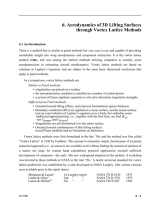
  • 24. 6 - 24 Applied Computational Aerodynamics To examine the use of these ideas we present a two-dimensional example. The airfoil is divided into a number of equal size panels. Each panel has a vortex at the quarter chord point and the non-penetration condition is satisfied at the three-quarter chord point. We use the example to illustrate the accuracy of the classical thin airfoil theory formulation. In Fig. 6-14, we compare the results obtained for a 5% circular arc camber.* Three solutions are presented. The linear theory curve uses classical thin airfoil theory with results obtained satisfying the boundary condition on the mean surface. This is compared with numerical results for the case where the boundary condition is applied exactly on the camber line, and the result obtained applying the boundary condition using the approximate method described above. The difference between placing the vortex on the actual camber surface and satisfying the boundary condition on the actual surface, and the more approximate traditional approach of locating the vortex and control point on the mean surface is extremely small. 3/11/98 0.90 0.80 0.70 0.60 0.50 0.40 0.30 0.20 0.10 DCp 5% Circular arc camber line a = 0 ° 40 panels 0.0 0.2 0.4 0.6 0.8 1.0 x/c DCp bc's on camber line DCp bc's on axis DCp linear theory Figure 6-14. Comparison in 2D of the 1/4-3/4 rule for vortex-control point locations with linear theory, and including a comparison between placing the vortex and control point on the camber line or on the axis. * A relatively large camber for a practical airfoil, the NACA 4412 example we used in Chapter 4 was an extreme case, and it has 4% camber.
  • 25. Aerodynamics of 3D Lifting Surfaces 6 - 25 6.7 The Classical Vortex Lattice Method There are many different vortex lattice schemes. In this section we describe the “classical” implementation. Knowing that vortices can represent lift from our airfoil analysis, and that one approach is to place the vortex and then satisfy the boundary condition using the “1/4 - 3/4 rule,” we proceed as follows: 3/11/98 1. Divide the planform up into a lattice of quadrilateral panels, and put a horseshoe vortex on each panel. 2. Place the bound vortex of the horseshoe vortex on the 1/4 chord element line of each panel. 3. Place the control point on the 3/4 chord point of each panel at the midpoint in the spanwise direction (sometimes the lateral panel centroid location is used) . 4. Assume a flat wake in the usual classical method. 5. Determine the strengths of each Gn required to satisfy the boundary conditions by solving a system of linear equations. The implementation is shown schematically in Fig. 6-15. y x X X X bound vortices X X control points X X X X Trailing vortices extend to infinity Figure 6-15. The horseshoe vortex layout for the classical vortex lattice method. Note that the lift is on the bound vortices. To understand why, consider the vector statement of the Kutta-Joukowski Theorem, F = rV ×G . Assuming the freestream velocity is the primary contributor to the velocity, the trailing vortices are parallel to the velocity vector and hence the force on the trailing vortices are zero. More accurate methods find the wake deformation required to eliminate the force in the presence of the complete induced flowfield.
  • 26. 6 - 26 Applied Computational Aerodynamics Next, we derive the mathematical statement of the classical vortex lattice method described above. First, recall that the velocity induced by a single horseshoe vortex is [ )k]× 3/11/98 Vm = Cm,nGn. (6-60) This is the velocity induced at the point m due to the nth horseshoe vortex, where Cm,n is a vector, and the components are given by Equations 6-54, 6-58 and 6-59. The total induced velocity at m due to the 2N vortices (N on each side of the planform) is: 2 N å . (6-83) Vmind = umind i + vmind j+ wmindk = Cm,nGn n=1 The solution requires the satisfaction of the boundary conditions for the total velocity, which is the sum of the induced and freestream velocity. The freestream velocity is (introducing the possibility of considering vehicles at combined angle of attack and sideslip): V¥ = V¥ cosa cosbi − V¥ sin bj + V¥ sina cosb k (6-84) so that the total velocity at point m is: Vm = (V¥ cosa cosb + umind ) i+ −V¥ sin b + vmind ( )j + (V¥sina cos b + wmind )k . (6-85) The values of the unknown circulations, Gn, are found by satisfying the non-penetration boundary condition at all the control points simultaneously. For steady flow this is V×n = 0 (6-1) where the surface is described by F(x, y,z) = 0. (6-86) Equation (6-1) can then be written: V× ÑF ÑF = V ×ÑF = 0 . (6-87) This equation provides freedom to express the surface in a number of forms. The most general form is obtained by substituting Eqn. (6-85) into Eqn. (6-87) using Eqn. (6-83). This can be written as: (V¥ cosa cosb + umind )i + −V¥ sinb + vmind ( )j + (V¥ sina cosb + wmind ¶F ¶ x i + ¶F ¶y j + ¶F ¶ z k é êë ù úû = 0 (6-88) or:
  • 27. Aerodynamics of 3D Lifting Surfaces 6 - 27 2N å )i + −V¥ sinb + Cm,njGn (V¥ cosa cos b + Cm,ni Gn 2N å =− V¥ cosa cosb 3/11/98 n=1 2Nå n=1 æ è çç ö ø 2Nå ÷÷ j + (V¥sina cosb + Cm,nk Gn n=1 )k é ë ê ê ù û ú ú × ¶F ¶ x i + ¶F ¶y j + ¶F ¶ z k é êë ù úû = 0 (6-89) Carrying out the dot product operation and collecting terms: ¶F ¶x 2N å )+ ¶F (V¥ cosa cosb + Cm,ni Gn n=1 ¶ y 2Nå −V¥ sin b + Cm,njGn n=1 æ è çç ö ø ÷÷ + ¶F ¶z 2Nå (V¥ sina cosb + Cm,nkGn n=1 ) = 0 . (6-90) Recall that Eqn. (6-90) is applied to the boundary condition at point m. Next, we collect terms to clearly identify the expression for the circulation. The resulting expression defines a system of equations for all the panels, and is the system of linear algebraic equations that is used to solve for the unknown values of the circulation distribution. The result is: ¶F ¶x Cm,ni + ¶F ¶ y Cm,nj + ¶F ¶ z Cm,nk æ ç è ö ø ÷ Gn n=1 ¶F ¶x − sinb ¶F ¶y + sina cos b ¶F ¶z é ëê ù úû m = 1,...2N (6-91) This is the general equation used to solve for the values of the circulation. It is arbitrary, containing effects of both angle of attack and sideslip (if the vehicle is at sideslip the trailing vortex system should by yawed to align it with the freestream). If the surface is primarily in the x-y plane and the sideslip is zero, we can write a simpler form. In this case the natural description of the surface is z = f(x, y) (6-92) and F(x, y,z) = z − f(x, y) = 0 . (6-93) The gradient of F becomes ¶F ¶x = − ¶f ¶x , ¶F ¶y = − ¶f ¶y , ¶F ¶z = 1. (6-94) Substituting into the statement of the boundary condition, Eqn. (6-91), we obtain: 2N å Cm,n − = Vk ¥ cosa ¶f ¶ x Cm,ni − ¶f ¶y Cm,n j é êë ù úû Gn n=1 ¶f ¶x − sina æ è ç ö ÷ , m = 1,...,2N . (6-95) ø This equation provides the solution for the vortex lattice problem.
  • 28. 6 - 28 Applied Computational Aerodynamics Note that if an essentially vertical surface is of interest, the form of F is more naturally To illustrate the usual method, consider the simple planar surface case, where there is no dihedral. Furthermore, recalling the example in the last section and the analysis at the beginning of the chapter, the thin airfoil theory boundary conditions can be applied on the mean surface, and not the actual camber surface. We also use the small angle approximations. Under these circumstances, Eq. (6-95) becomes: 3/11/98 2Nå wm = Cm,nk Gn n=1 = V¥ æ − a è ç ö dfc dx ÷ m ø . (6-96) Thus we have the following equation which satisfies the boundary conditions and can be used to relate the circulation distribution and the wing camber and angle of attack: 2N å = dfc Cm,nk æ è Gn V¥ ç ö ÷ ø n=1 æ −a è ç ö dx ÷ m ø m = 1,...,2N. (6-97) Equation (6-97) contains two cases: 1. The Analysis Problem. Given camber slopes and a, solve for the circulation strengths, (G/V¥) [ a system of 2N simultaneous linear equations]. or 2. The Design Problem. Given (G/V¥), which corresponds to a specified surface loading, we want to find the camber and a required to generate this loading (only requires simple algebra, no system of equations must be solved). Notice that the way dfc/dx and a are combined illustrates that the division between camber, angle of attack and wing twist is arbitrary (twist can be considered a separate part of the camber distribution, and is useful for wing design). However, care must be taken in keeping the bookkeeping straight. One reduction in the size of the problem is available in many cases. If the geometry is symmetrical and the camber and twist are also symmetrical, then Gn is the same on each side of the planform (but not the influence coefficient). Therefore, we only need to solve for N G’s, not 2N (this is true also if ground effects are desired, see Katz and Plotkin11). The system of equations for this case becomes: é ëê Cm,nkleft + Cm,nkright æ è ù úû Nå n=1 Gn V¥ ç ö ø æ −a è ç ö ÷ = dfc dx ÷ m ø m = 1,...,N. (6-98) F = y - g(x,z), and this should be used to work out the boundary condition in a similar fashion.
  • 29. Aerodynamics of 3D Lifting Surfaces 6 - 29 This is easy. Why not just program it up ourselves? You can, but most of the work is: 3/11/98 A. Automatic layout of panels for arbitrary geometry. As an example, when considering multiple lifting surfaces, the horseshoe vortices on each surface must “line up”. The downstream leg of a horseshoe vortex cannot pass through the control point of another panel. and B. Converting Gn to the aerodynamics values of interest, CL, Cm, etc., and the spanload, is tedious for arbitrary configurations. Nevertheless, many people (including previous students in the Applied Computational Aerodynamics class) have written vlm codes. The method is widely used in industry and government for aerodynamic estimates for conceptual and preliminary design predictions. The method provides good insight into the aerodynamics of wings, including interactions between lifting surfaces. Typical analysis uses (in a design environment) include • Predicting the configuration neutral point during initial configuration layout, and studying the effects of wing placement and canard and/or tail size and location. • Finding the induced drag, CDi, from the spanload in conjunction with farfield methods. • With care, estimating control and device deflection effectiveness (estimates where viscous effects may be important require calibration. Some examples are shown in the next section. For example, take 60% of the inviscid value to account for viscous losses, and also realize that a deflection of df = 20 - 25° is about the maximum useful device deflection in practice). • Investigating the aerodynamics of interacting surfaces. • Finding the lift curve slope, CLa, approach angle of attack, etc. Typical design applications include: • Initial estimates of twist to obtain a desired spanload, or root bending moment. • Starting point for finding a camber distribution in purely subsonic cases. Before examining how well the method works, two special cases require comments. The first case arises when a control point is in line with the projection of one of the finite length vortex segments. This problem occurs when the projection of a swept bound vortex segment from one side of the wing intersects a control point on the other side. This happens frequently. The velocity induced by this vortex is zero, but the equation as usually written degenerates into a singular form, with the denominator going to zero. Thus a special form should be used. In practice, when this happens the contribution can be set to zero without invoking the special form. Figure 6-16 shows how this happens. Using the Warren 12 planform and 36 vortices on each side of the wing, we see that the projection of the line of bound vortices on the last row of the left hand side of the planform has a projection that intersects one of the control points on the right hand side.
  • 30. 6 - 30 Applied Computational Aerodynamics 3/11/98 -0.50 0.00 0.50 1.00 1.50 2.00 2.50 3.00 Warren 12 planform example is for 36 horseshoe projection of bound vortices on this row intersect control point on other side of planform horseshoe vortex vortices on each side, all vortices not shown for clarity control point trailing legs extend to infinity -2.0 -1.5 -1.0 -0.5 0.0 0.5 1.0 1.5 2.0 Figure 6-16. Example of case requiring special treatment, the intersection of the projection of a vortex with a control point. A model problem illustrating this can be constructed for a simple finite length vortex segment. The velocity induced by this vortex is shown in Fig. 6-17. When the vortex is approached directly, x/l = 0.5, the velocity is singular for h = 0. However, as soon as you approach the axis (h = 0) off the end of the segment (x/l > 1.0) the induced velocity is zero. This illustrates why you can set the induced velocity to zero when this happens. This second case that needs to be discussed arises when two or more planforms are used with this method. This is one of the most powerful applications of the vortex lattice method. However, care must be taken to make sure that the trailing vortices from the first surface do not intersect the control points on the second surface. In this case the induced velocity is in fact infinite, and the method breaks down. Usually this problem is solved by using the same spanwise distribution of horseshoe vortices on each surface. This aligns the vortex the legs, and the control points are well removed from the trailing vortices of the forward surfaces.
  • 31. Aerodynamics of 3D Lifting Surfaces 6 - 31 3/11/98 1.00 0.80 0.60 0.40 0.20 0.00 x/l x 0.0 0.5 1.0 1.5 2.0 Vp h/l 0.5 1.5 2.0 3.0 h p l x=0 Figure 6-17. Velocity induced by finite straight line section of a vortex.
  • 32. 6 - 32 Applied Computational Aerodynamics 6.8 Examples of the Use and Accuracy of the vlm Method How well does the method work? In this section we describe how the method is normally applied, and present some example results obtained using it. More examples and a discussion of the aerodynamics of wings and multiple lifting surfaces are given in Section 6.10. The vortex lattice layout is clear for most wings and wing-tail or wing-canard configurations. The method can be used for wing-body cases by simply specifying the projected planform of the entire configuration as a flat lifting surface made up of a number of straight line segments. The exact origin of this somewhat surprising approach is unknown. The success of this approach is illustrated in examples given below. To get good, consistent and reliable results some simple rules for panel layout should be followed. This requires that a few common rules of thumb be used in selecting the planform break points: i) the number of line segments should be minimized, ii) breakpoints should line up streamwise on front and rear portions of each planform, and should line up between planforms, iii) streamwise tips should be used, iv) small spanwise distances should be avoided by making edges streamwise if they are actually very highly swept, and v) trailing vortices from forward surfaces cannot hit the control point of an aft surface. Figure 6-18 illustrates these requirements. 3/11/98 Make edges streamwise y first planform second planform x line up spanwise breaks on a common break, and make the edge streamwise Model Tips • start simple • crude representation of the planform is all right • keep centroids of areas the same: actual planform to vlm model Figure 6-18. Example of a vlm model of an aircraft configuration. Note that one side of a symmetrical planform is shown.
  • 33. Aerodynamics of 3D Lifting Surfaces 6 - 33 Examples from three reports have been selected to illustrate the types of results that can be expected from vortex lattice methods. They illustrate the wide range of uses for the vlm method. Aircraft configurations examined by John Koegler15 As part of a study on control system design methods, John Koegler at McDonnell Aircraft Company studied the prediction accuracy of several methods for fighter airplanes. In addition to the vortex lattice method, he also used the PAN AIR and Woodward II panel methods (see Chapter 4 for details of the panel methods). He compared his predictions with the three-surface F-15, which became known as the STOL/Maneuver demonstrator, and the F-18. These configurations are illustrated in Fig. 6-19. 3/11/98 Three-Surface F-15 F/A-18 Figure 6-19. Configurations used by McDonnell Aircraft to study vlm method accuracy (Reference 15).
  • 34. 6 - 34 Applied Computational Aerodynamics Considering the F-15 STOL/Maneuver demonstrator first, the basic panel layout is given in Figure 6-20. This shows how the aircraft was modeled as a flat planform, and the corner points of the projected configuration were used to represent the shape in the vortex lattice method and the panel methods. Note that in this case the rake of the wingtip was included in the computational model. In this study the panel methods were also used in a purely planar surface mode. In the vortex lattice model the configuration was divided into three separate planforms, with divisions at the wing root leading and trailing edges. On this configuration each surface was at a different height and, after some experimentation, the vertical distribution of surfaces shown in Figure 6-21 was found to provide the best agreement with wind tunnel data. 3/11/98 Vortex Lattice 233 panels Woodward 208 panels Pan Air 162 panels Figure 6-20. Panel models used for the three-surface F-15 (Ref.15). Figure 6-21. Canard and horizontal tail height representation (Ref. 15).
  • 35. Aerodynamics of 3D Lifting Surfaces 6 - 35 The results from these models are compared with wind tunnel data in Table 6-1. The vortex lattice method is seen to produce excellent agreement with the data for the neutral point location, and lift and moment curve slopes at Mach 0.2. Subsonic Mach number effects are simulated in vlm methods by transforming the Prandtl- Glauert equation which describes the linearized subsonic flow to Laplace’s Equation using the Göthert transformation. However, this is only approximately correct and the agreement with wind tunnel data is not as good at the transonic Mach number of 0.8. Nevertheless, the vlm method is as good as PAN AIR used in this manner. The vlm method is not applicable at supersonic speeds. The wind tunnel data shows the shift in the neutral point between subsonic and supersonic flow. The Woodward method, as applied here, over predicted the shift with Mach number. Note that the three-surface configuration is neutral to slightly unstable subsonically, and becomes stable at supersonic speeds. Figure 6-22 provides an example of the use of the vlm method to study the effects of moving the canard. Here, the wind tunnel test result is used to validate the method and to provide an “anchor” for the numerical study (it would have been useful to have to have an experimental point at -15 inches). This is typical of the use of the vlm method in aircraft design. When the canard is above the wing the neutral point is essentially independent of the canard height. However when the canard is below the wing the neutral point varies rapidly with canard height. 3/11/98 M = 0.2 M = 0.8 M = 1.6 Wind Tunnel Vortex Lattice Woodward Pan Air Wind Tunnel Vortex Lattice Pan Air Wind Tunnel Woodward Table 6-1 Three-Surface F-15 Longitudinal 1Derivatives Neutral Point (% mac) Cma (1/deg) CLa (1/deg) Data Source 15.70 .00623 .0670 15.42 .00638 .0666 14.18 .00722 .0667 15.50 .00627 .0660 17.70 .00584 .0800 16.76 .00618 .0750 15.30 .00684 .0705 40.80 -.01040 .0660 48.39 -.01636 .0700 from reference 15, Appendix by John Koegler
  • 36. 6 - 36 Applied Computational Aerodynamics 3/11/98 16 12 8 Neutral Point percent c CLa per deg -20 -10 0 10 20 Canard Height, in. 0.07 0.06 Vortex lattice Wind tunnel data Figure 6-22. Effect of canard height variation on three-surface F-15 characteristics (Ref. 15). Control effectiveness is also of interest in conceptual and preliminary design, and the vlm method can be used to provide estimates. Figure 6-23 provides an apparently accurate example of this capability for F-15 horizontal tail effectiveness. Both CLdh and Cmdh are presented. The vlm estimate is within 10% accuracy at both Mach .2 and .8. However, the F-15 has an all moving horizontal tail to provide sufficient control power under both maneuvering and supersonic flight conditions. Thus the tail effectiveness presented here is effectively a measure of the accuracy of the prediction of wing lift and moment change with angle of attack in a non-uniform flowfield, rather than the effectiveness of a flap-type control surface. A flapped device such as a horizontal stabilizer and elevator combination will have significantly larger viscous effects, and the inviscid estimate from a vortex lattice or panel method (or any inviscid method) will overpredict the control effectiveness. This is shown next for an aileron. The aileron effectiveness for the F-15 presented in Fig. 6-24 is more representative of classical elevator or flap effectiveness correlation between vlm estimates and experimental data. This figure presents the roll due to aileron deflection. In this case the device deflection is subject to significant viscous effects, and the figure shows that only a portion of the effectiveness predicted by the vlm method is realized in the actual data. The vlm method, or any method, should always be calibrated with experimental data close to the cases of interest to provide an indication of the agreement between theory and experiment. In this case the actual results are found to be about 60% of the inviscid prediction at low speed.
  • 37. Aerodynamics of 3D Lifting Surfaces 6 - 37 3/11/98 -0.02 0.0 0.4 0.8 1.2 1.6 2.0 Mach Number 0.02 0.01 0.00 Wind tunnel Vortex lattice Woodward CmdH per deg. CLdH per deg. -0.01 0.00 Figure 6-23. F-15 horizontal tail effectiveness (Ref. 15). 0.0 0.2 0.4 0.6 0.8 1.0 Mach Number 0.0016 0.0012 0.0008 0.0004 Clda 0.0000 Wind tunnel Vortex lattice:Sym Wing chordwise panels 68 10 per deg. (da = ± 20°) Figure 6-24. F-15 aileron effectiveness (Ref. 15).
  • 38. 6 - 38 Applied Computational Aerodynamics The F/A-18 was also considered by Koegler. In this case the contributions to the longitudinal derivatives by the wing-tip missiles and the vertical tail were investigated (the vertical tails are canted outward on the F/A-18). The panel scheme used to estimate the effects of the wing-tip missile and launcher is shown in Figure 6-25. The results are given in Table 6-2. Here the computational increments are compared with the wind tunnel increments. The vlm method over predicts the effect of the wing-tip missiles, and under predicts the effects of the contribution of the vertical tail to longitudinal characteristics due to the cant of the tail (recall that on the F/A-18 the rudders are canted inward at takeoff to generate an additional nose up pitching moment) . 3/11/98 Figure 6-25. F/A-18 panel scheme with wing-tip missile and launcher (Ref. 15).
  • 39. Aerodynamics of 3D Lifting Surfaces 6 - 39 3/11/98 Wing Tip Missiles and Launchers Vertical Tails Wind Tunnel " " Vortex Lattice " Woodward " " Wind Tunnel " Vortex Lattice " Table 6-2 F/A-18 Increments Due To Adding Wing-Tip Missiles and Launchers, and Vertical Tails Mach Number DNeutral Point (% mac) DCMa (1/deg) DCLa (1/deg) 0.2 1.10 -0.00077 0.0020 0.8 1.50 -0.00141 0.0030 1.6 -1.60 0.00148 0.0030 0.2 1.48 -0.00121 0.0056 0.8 2.11 -0.00198 0.0082 0.2 1.52 -0.00132 0.0053 0.8 1.77 -0.00180 0.0079 1.6 -0.17 0.00074 0.0022 0.2 1.50 -0.00110 0.0050 0.8 2.00 -0.00202 0.0080 0.2 1.11 -0.00080 0.0022 0.8 1.32 -0.00108 0.0026 from refernce 15, Appendix by John Koegler Finally, the effects of the number of panels and the way they are distributed is presented in Figure 6-26. In this case the vlm method is seen to take between 130 to 220 panels to produce converged results. For the vortex lattice method it appears important to use a large number of spanwise rows, and a relatively small number of chordwise panels (5 or 6 appear to be enough).
  • 40. 6 - 40 Applied Computational Aerodynamics 3/11/98 4 2 0 ( ) Number of chordwise panels (5) (9) Vortex Lattice Method 0 40 80 120 160 200 240 Total number of panels D Neutral point, percent c a) vortex lattice sensitivity to number of panels 6 4 2 0 (4) 0 40 80 120 160 200 240 Total number of panels Woodward Program (8) ( ) Number of chordwise panels D Neutral point, percent c b) Woodward program sensitivity to number of panels 0 -2 0 40 80 120 160 200 240 Total number of panels Pan Air (3) ( ) Number of chordwise panels D Neutral point, percent c c) Pan Air program sensitivity to number of panels Figure 6-26. F/A-18 panel convergence study (Ref. 15). Although this study has been presented last in this section, a study like this should be conducted before making a large number of configuration parametric studies. Depending on the relative span to length ratio the paneling requirements may vary. The study showed that from about 120 to 240 panels are required to obtain converged results. The vortex lattice methods obtains the best results when many spanwise stations are used, together with a relatively small number of chordwise panels. In that case about 140 panels provided converged results.
  • 41. Aerodynamics of 3D Lifting Surfaces 6 - 41 Slender lifting body results from Jim Pittman16 To illustrate the capability of the vortex lattice method for bodies that are more fuselage-like than wing-like, we present the lifting body comparison of the experimental and vlm results published by Jim Pittman of NASA Langley. Figure 6-27 shows the configuration used. Figure 6-28 provides the results of the vortex lattice method compared with the experimental data. In this case the camber shape was modeled by specifying camber slopes on the mean surface. The model used 138 vortex panels. The bars at several angles of attack illustrate the range of predictions obtained with different panel arrangements. For highly swept wings, leading edge vortex flow effects are included, as we will describe in Section 6.12. The program VLMpc available for this course contains the option of using the leading edge suction analogy to model these effects. Remarkably good agreement with the force and moment data is demonstrated in Fig. 6-28. The nonlinear variation of lift and moment with angle of attack arises due to the inclusion of the vortex lift effects. The agreement between data and computation breaks down at higher angles of attack because the details of the distribution of vortex flow separation are not provided by the leading edge suction analogy. The drag prediction is also very good. The experimental drag is adjusted by removing the zero lift drag, which contains the drag due to friction and separation. The resulting drag due to lift is compared with the vlm estimates. The comparisons are good primarily because this planform is achieving, essentially, no leading edge suction, and hence the drag is simply CD = CLtana. 3/11/98 copyrighted figure from the AIAA Journal of Aircraft Figure 6-27. Highly swept lifting body type hypersonic concept (Ref. 16).
  • 42. 6 - 42 Applied Computational Aerodynamics 3/11/98 copyrighted figure from the AIAA Journal of Aircraft Figure 6-28. Comparison of CL, Cm, and CD predictions with data (Ref. 16). Non-planar results from Kalman, Rodden and Giesing,17 All of the examples presented above considered essentially planar lifting surface cases. The vortex lattice method can also be used for highly non-planar analysis, and the example cases used at Douglas Aircraft Company in a classic paper17 have been selected to illustrate the capability. To avoid copyright problems, several of the cases were re-computed using the Virginia Tech code JKayVLM, and provide an interesting comparison with the original results from Douglas. Figure 6-29 presents an example of the prediction capability for the pressure loading on a wing. In this case the geometry is complicated by the presence of a wing fence. The pressures are compared with data on the inboard and outboard sides of the fence. The agreement is very good on the inboard side. The comparison is not so good on the outboard side of the fence. This quality of agreement is representative of the agreement that should be expected using vortex lattice methods at low Mach numbers in cases where the flow would be expected to be attached. Figure 6-30 provides an example of the results obtained for an extreme non-planar case: the ring, or annular, wing. In this case the estimates are compared with other theories, and seen to be very good. The figure also includes the estimate of Cmq. Although not included in the present discussion, Cmq and Clp can be computed using vlm methods, and this capability is included in the vortex lattice method provided here, VLMpc.
  • 43. Aerodynamics of 3D Lifting Surfaces 6 - 43 3/11/98 copyrighted figure from the AIAA Journal of Aircraft Figure 6-29. Comparison of DCp loading on a wings with a fence (Ref. 17). copyrighted figure from the AIAA Journal of Aircraft Figure 6-30. Example of aerodynamic characteristics of a ring wing (Ref. 17).
  • 44. 6 - 44 Applied Computational Aerodynamics Figure 6-31 provides an example of the effects of the presence of the ground on the aerodynamics of simple unswept rectangular wings. The lift and pitching moment slopes are presented for calculations made using JKayVLM and compared with the results published by Kalman, Rodden and Giesing,17 and experimental data. The agreement between the data and calculations is excellent for the lift curve slope. The AR = 1 wing shows the smallest effects of ground proximity because of the three dimensional relief provided around the wing tips. As the aspect ratio increases, the magnitude of the ground effects increases. The lift curve slope starts to increase rapidlyi as the ground is approached. 3/11/98 8.0 7.0 6.0 5.0 4.0 3.0 2.0 1.0 0.0 0.2 0.4 0.6 0.8 1.0 1.2 1.4 CLa h/c AR 4 2 1 Solid lines: computed using JKayVLM (Ref. 12) Dashed lines: from Kalman, Rodden and Giesing (Ref. 17) Symbols: Experimental data h U¥ c c/4 0.20 0.10 0.00 -0.10 -0.20 -0.30 -0.40 Solid lines: computed using JKayVLM (Ref. 12) Dashed lines: from Kalman, Rodden and Giesing (Ref. 17) 0.0 0.2 0.4 0.6 0.8 1.0 1.2 1.4 CMa h/c AR 1 2 4 Figure 6-31. Example of ground effects for a simple rectangular wing (a case from Ref. 17). The wings also experience a significant change in the pitching moment slope (aerodynamic center shift), and this is also shown. Note that the predictions start to differ as the ground is approached. JKayVLM actually rotates the entire surface to obtain another solution to use in estimating the lift curve slope. The standard procedure used by most methods is to simply change the slope condition at the mean line, as discussed previously in this chapter. Because of
  • 45. Aerodynamics of 3D Lifting Surfaces 6 - 45 the proximity to the ground, this might be a case where the transfer of the boundary condition may not be accurate. I have not asked Joe Giesing if he remebers how these calculations were made (nearly 30 years ago!). Figure 6-32 presents similar information for the effect of dihedral angle on a wing. In this case the effects of anhedral, where the wing tip approach the ground, are extremely large. The results of dihedral changes for a wing out of ground effect are shown for comparison. Both methods agree well with each other, with differences appearing only as the wingtips approach the ground. Here again, JKayVLM actually rotates the entire geometry, apparently resulting in an increase in the effects as the tips nearly contact the ground. It also prevents calculations from being obtained as close to the ground as thepublished results. In making these calculations it was discovered that the wing panel was rotated and not sheared, so that the projected span decreases as the dihedral increases, and this produces much more pronounced changes in the lift curve slope due to the reduction in projected span. 3/11/98 12 10 8 6 4 2 0 Solid lines: computed using JKayVLM (Ref. 12) Dashed lines: from Kalman, Rodden and Giesing (Ref. 17) ARref = 4, Planform rotated by G. h/c = 0.5 h/c = 1 h/c = ¥ Note: Most of the decrease in lift curve slope for the wing out of ground effect is due to the effect of reduced span as the wing rotates from the zero dihedral condition -40° -30° -20° -10° 0° 10° 20° 30° 40° CLa Dihedral angle, G G h Figure 6-32. Example of ground effects for a wing with dihedral (a case from Ref. 17).
  • 46. 6 - 46 Applied Computational Aerodynamics 6.9 Program VLMpc and the Warren 12 Test Case This vortex lattice method can be used on personal computers. The version of the Lamar program described in NASA TN D-79213 fits easily into personal computers, and is available for student use (students typed this code in from the listing in the TN) as VLMpc. The code and input instructions are described in Appendix D.6. This code is still used in advanced design work, and can be used to investigate many ideas in wing aerodynamics. As shown above, results can be obtained and used before the large time consuming methods of CFD are used to examine a particular idea in detail. This section defines one reference wing case that is used to check the accuracy of vortex lattice codes. It provides a ready check case for the evaluation of any new or modified code, as well as a check on the panel scheme layout. This wing is known as the Warren 12 planform, and is defined, together with the “official” characteristics from previous calculations, in Fig. 6-33 below. 3/11/98 1.50 0.50 1.41421 1.91421 Warren-12 Planform AR = 2 2 LLE = 53.54° Swing = 2 2 CLa = 2.743 / rad CMa = −3.10 / rad Figure 6-33. Definition and reference results for the Warren-12 wing. For the results cited above, the reference chord used in the moment calculation is the average chord (slightly nonstandard, normally the reference chord used is the mean aerodynamic chord) and the moment reference point is located at the wing apex (which is also nonstandard).
  • 47. Aerodynamics of 3D Lifting Surfaces 6 - 47 6.10 Aerodynamics of Wings With a three-dimensional method available, we can examine the aerodynamics of wings. Most of the results presented in this section were computed using VLMpc. One key advantage of the vortex lattice method compared to lifting line theory is the ability to treat swept wings. Classical Prandtl lifting line theory is essentially correct for unswept wings, but is completely erroneous for swept wings. Aerodynamics of unswept wings are closely related to the airfoil characteristics of the airfoil used in the wing. This relationship is less direct for swept wings. Many of the most important wing planform-oriented characteristics of wings arise when the planforms are swept. Even though sweep is used primarily to reduce compressibility effects, the important aerodynamic features of swept wings can be illustrated at subsonic speeds using the vlm method. 6.10.1 - Basic Ideas Wings are designed to satisfy stability and handling characteristics requirements, while achieving low drag at the design conditions (usually cruise and sustained maneuver). They must also attain high maximum lift coefficients to meet field performance and maneuver requirements. Although these requirements might at first appear overwhelming, a small number of key characteristics can provide a basic physical understanding of the aerodynamics of wings. Aerodynamic Center: The first key characteristic is the aerodynamic center of the wing, defined as location at which dCm/dCL = 0. The neutral point of the configuration is the aerodynamic center for the entire configuration. The vlm method was shown to provide accurate predictions of the neutral point for many configurations in the previous sections. The location of the neutral point is important in initial configuration layout to position the wing and any longitudinal stability and control surfaces at the proper location on the aircraft. Subsequently this information is fundamental in developing the control system. Wing planform shaping, as well as positioning, is used to control the location of the configuration neutral point. Spanload: The next key consideration is the spanload distribution, ccl/ca, where c is the local chord, ca is the average chord, and cl is the local section lift coefficient. The spanload controls the location of the maximum section lift coefficient, the induced drag, and the magnitude of the wing root bending moment. The location and value of the maximum section lift coefficient determines where the wing will stall first.* If the wing airfoil stalls in front of a control surface, control will be poor at flight conditions where the control becomes very important. The shape of the spanload, together with the actual value of the wingspan, determines the value of the induced * For a trapezoidal wing with an elliptic spanload the maximum value of the local lift coefficient occurs at h = 1 - l. 3/11/98
  • 48. 6 - 48 Applied Computational Aerodynamics drag. For a specified span, the performance of the wing is evaluated by finding the value of the span efficiency factor, e, as described in Chapter 5. Finally, the wing root bending moment provides an indication of the structural loading requirements that the wing structure must be designed to accommodate. When considering the total system, the basic aerodynamic efficiency may be compromised to reduce structural wing weight. The shape of the spanload can be controlled through a combination of planform selection and wing twist. Typical twist distributions required to produce good wing characteristics are presented below. The simplest example of planform shaping is the selection of wing aspect ratio, AR, wing taper, l, and wing sweep, L. While the aerodynamicist would like to see high values the aspect ratio, several considerations limit aspect ratio. Perhaps the most important limitation is the increase of wing structural weight with increasing aspect ratio. In addition, the lift coefficient required to maximize the benefits of high aspect ratio wings increases with the square root of the aspect ratio. Hence, airfoil performance limits can restrict the usefulness of high aspects ratios, especially for highly swept wings based on airfoil concepts. In recent years advances in both aerodynamics and structures have allowed aircraft to be designed with higher aspect ratios and reduced sweep. Table 6-3 provides some key characteristics of transport wings designed to emphasize efficient cruise while meeting takeoff and landing requirements. Taper: Several considerations are used in selecting the wing taper. For a straight untwisted, unswept wing, the minimum induced drag corresponds to a taper ratio of about 0.4. However, a tapered wing is more difficult and hence expensive to build than an untapered wing. Many general aviation aircraft wings are built with no taper (all ribs are the same, reducing fabrication cost, and the maximum section Cl occurs at the root, well away from the control surface). To reduce structural weight the wing should be highly tapered, with l < .4. However, although highly tapered wings are desirable structurally, the section lift coefficient near the tip may become high. This consideration limits the amount of taper employed (current jet transports use taper ratios in the range of 0.2 to 0.3, as well as progressively increasing twist upward from the tip). As an example, the Aero Commander 500 had an aspect ratio of 9.5 and a taper ratio of 0.5 (it also had -6.5° of twist and the quarter chord of the wing was swept forward 4°). Sweep: Sweep is used primarily to delay the effects of compressibility and increase the drag divergence Mach number. The Mach number controlling these effects is approximately equal to the Mach number normal to the leading edge of the wing, Meff = M¥cosL. The treatise on swept planforms by Küchemann is very helpful in understanding swept wing aerodynamics.18 Aerodynamic performance is based on the wingspan, b. For a fixed span, the structural span increases with sweep, bs = b/cosL, resulting in a higher wing weight. Wing sweep also leads to aeroelastic problems. For aft swept wings flutter becomes an important consideration. If the wing 3/11/98
  • 49. Aerodynamics of 3D Lifting Surfaces 6 - 49 is swept forward, divergence is a problem. Small changes in sweep can be used to control the aerodynamic center when it is not practical to adjust the wing position on the fuselage (the DC-3 is the most famous example of this approach). 3/11/98 1957 1958 1963 1970 1970 1972 1972 1982 1986 1988 1990 1992 Table 6-3 Typical Planform Characteristics of Major Transport Aircraft 1st Flight Aircraft W/S AR L °(c/4) l B707-120 105.6 7.04 35 0.293 DC-8-10 111.9 7.32 30 0.230 B707-320C 110.0 7.06 35 0.250 B747-200B 149.1 6.96 37.5 0.240 L-1011 124.4 8.16 35 0.200 DC-10-30 153.7 7.57 35 0.230 A300 B2 107.9 7.78 28 0.230 A310-100 132.8 8.80 28 0.260 B767-300 115.1 7.99 31.5 0.182 B747-400 149.9 7.61 37.5 0.240 MD-11 166.9 7.57 35 0.230 A330 119.0 9.3 29.74 0.192 data courtesy of Nathan Kirschbaum To understand the effects of sweep, the Warren 12 wing is compared with wings of the same span and aspect ratio, but unswept and swept forward. The planforms are shown in Figure 6-34. The wing leading edge sweep of the aft swept wing becomes the trailing edge sweep of the forward swept wing. Figure 6-35 provides the spanload and section lift coefficient distributions from VLMpc. The spanload, ccl / ca , is given in Fig. 6-35a, where, c is the local chord, cl is the local lift coefficient, based on the local chord, and ca is the average chord, S/b. Using this nomenclature, the area under the curve is the total wing lift coefficient. Note that sweeping the wing aft increases the spanload outboard, while sweeping the wing forward reduces the spanload outboard. This follows directly from a consideration of the vortex lattice model of the wing. In both cases, the portion of the wing aft on the planform is operating in the induced upwash flowfield of the wing ahead of it, resulting in an increased spanload. Figure 6-35b shows the corresponding value of the local lift coefficient. Here the effect of sweep is more apparent. The forward swept wing naturally results in a spanload with a nearly constant lift coefficient. This means that a comparatively higher wing lift coefficient can be achieved before the wing stall begins. The program LIDRAG can be used to compare the span e’s associated with these spanloads (an exercise for the reader).
  • 50. 6 - 50 Applied Computational Aerodynamics 3/11/98 V¥ Forward Swept Wing Unswept Wing Aft Swept Wing Figure 6-34. Comparison of forward, unswept, and aft swept wing planforms, AR = 2.8.
  • 51. Aerodynamics of 3D Lifting Surfaces 6 - 51 3/11/98 1.60 1.40 1.20 1.00 0.80 0.60 0.40 0.20 0.00 aft swept wing unswept wing forward swept wing 0.0 0.2 0.4 0.6 0.8 1.0 y/(b/2) Spanload, Warren 12 planform, sweep changed c c l / c a a) comparison of spanloads 1.40 1.20 1.00 0.80 0.60 0.40 0.20 0.00 aft swept wing unswept wing forward swept wing 0.0 0.2 0.4 0.6 y/(b/2) 0.8 1.0 Section CL Warren 12 planform, sweep changed b) comparison of section lift coefficients Figure 6-35. Effects of sweep on planform spanload and lift coefficient distributions, AR = 2.8.
  • 52. 6 - 52 Applied Computational Aerodynamics Similar results are now presented for a series of wings with larger aspect ratios (AR = 8) than the wings used in the study given above. Figure 6-36 shows the planforms used for comparison, and Figure 6-37 presents the results for the spanwise distribution of lift and section lift coefficient. These results are similar to the previous results. However, the trends observed above are in fact exaggerated at the higher aspect ratio. Aerodynamic problems as well as structural penalties arise when using a swept wing. Because of the high section lift coefficient near the tip, aft swept wings tend to stall near the tip first. Since the lift at the tip is generated well aft, the pitching moment characteristics change when the this stall occurs. With the inboard wing continuing to lift, a large positive increase in pitching moment occurs when the wingtip stalls. This is known as pitchup, and can be difficult to control, resulting in unsafe flight conditions. Frequently the swept wing pitching moment characteristics are compounded by the effects of flow separation on the outboard control surface. Figure 6-38 provides an example of the pitching moment characteristics of an isolated aspect ratio 10 wing using experimental data.19 The figure also includes the predictions from VLMpc. The agreement is reasonably good at low angle of attack, but deteriorates at high angle of attack as viscous effects become important. This is another reason that sweep is minimized. 3/11/98 V¥ Forward Swept Wing Unswept Wing Aft Swept Wing Figure 6-36. Comparison of forward, unswept, and aft swept wing planforms, AR = 8.
  • 53. Aerodynamics of 3D Lifting Surfaces 6 - 53 3/11/98 1.6 1.4 1.2 1.0 0.8 0.6 0.4 0.2 0.0 0.2 0.4 0.6 0.8 1.0 Spanload, y/(b/2) Aspect ratio 8 wings aft swept wing unswept wing forward swept wing cc l / c a a) comparison of spanloads 1.50 1.00 0.50 0.00 aft swept wing unswept wing forward swept wing 0.0 0.2 0.4 0.6 Section CL 0.8 1.0 Aspect ratio 8 planforms y/(b/2) b) comparison of section lift coefficients Figure 6-37. Effects of sweep on planform spanload and lift coefficient distributions, AR = 8.
  • 54. 6 - 54 Applied Computational Aerodynamics 3/11/98 0.08 0.06 0.04 0.02 0.00 -0.02 -0.04 -0.06 data from NACA RM A50K27 AR = 10, Lc/4 = 35°, l = 0.5 Re = 10 million x ref = c/4 VLMpc calculation -0.4 -0.2 0.0 0.2 0.4 0.6 0.8 1.0 1.2 Cm CL Figure 6-38. Example of isolated wing pitchup: NACA data19 compared with VLMpc. To control the spanload, the wing can be twisted. Figure 6-39 shows typical twist distributions for aft and forward swept wings, obtained from John Lamar’s program LamDes.20 (see Chapter 5 for a description). In each case the twist is used to reduce the highly loaded areas, and increase the loading on the lightly loaded portions of the wing. For an aft swept wing this means the incidence is increased at the wing root, known as washin, and reduced, known as washout, at the wing tip. Just the reverse is true for the forward swept wing. The sudden drop in required twist at the tip for the forward dwept wing case is frequently seen in typical design methods and attribute to a weakness in the method and “faired out” when the aerodynamicist gives his design to the lofting group. Although geometric sweep is used to reduce the effective Mach number of the airfoil, the geometric sweep is not completely effective. The flowfield resists the sweep. In particular, the wing root and tip regions tend to effectively unsweep the wing. Aerodynamicists study lines of constant pressure on the wing planform known as isobars to investigate this phenomenon. Figure 6-40 presents the computed isobars for a typical swept wing,21 using a transonic small disturbance method.22 The effect is dramatic. The effective sweep may actually correspond to the isobar line from the wing root trailing edge to the leading edge at the wing tip. To increase the isobar sweep, in addition to geometric sweep and twist, the camber surface and thickness are typically adjusted to move the isobars forward at the wing root and aft at the wing tip. This is a key part of the aerodynamic wing design job, regardless of the computational, methodology used to obtain the predicted isobar pattern.
  • 55. Aerodynamics of 3D Lifting Surfaces 6 - 55 6.0 5.0 4.0 3.0 2.0 1.0 0.0 -1.0 AR = 4 l = 0.6 3/11/98 0 0.2 0.4 0.6 0.8 1 q, deg. y/(b/2) 7.0 6.0 5.0 4.0 3.0 2.0 1.0 0.0 -1.0 0 0.2 0.4 0.6 0.8 1 q, deg. y/(b/2) a) aft swept wing b) forward swept wing Figure 6-39. Typical twist distribution required to improve spanload on swept wings (b) Upper Surface Isobars 45° (a) L51F07 configuration Figure 6-40. Example of the isobar distribution on an untwisted swept wing.22 Using the wing planform and twist, together with a constant chord loading, Fig. 6-41 provides the camber lines required to support the load near the root, the mid-span and the wing tip. These results were also computed using LamDes.20 At each station a similar chord load is specified. Here we clearly see the differences in the camber required. This is an explicit illustration of the modification to an airfoil camberline required to maintain two-dimensional airfoil-type performance when the airfoil is placed in a swept wing. These modifications represent the explicit effects of the three dimensionality of the flowfield.
  • 56. 6 - 56 Applied Computational Aerodynamics 3/11/98 0.05 0.04 0.03 0.02 0.01 0.00 -0.01 -0.2 0 0.2 0.4 0.6 0.8 1 1.2 (z-zle)/c x/c h = 0.925 h = 0.475 h = 0.075 Figure 6-41. Comparison of camber lines required to develop the same chord load shape at the root, mid-span and tip region of an aft swept wing. (from LamDes20) Many other refinements are available to the aerodynamic designer. Insight into both the human and technical aspects of wing design prior to the introduction of computational aerodynamics is available in two recent books describing the evolution of the Boeing series of jet transports.23,24 One interesting refinement of swept wings has been the addition of trailing edge area at the wing root. Generally known as a “Yehudi flap”, this additional area arises for at least two reasons. The reason cited most frequently is the need to provide structure to attach the landing gear at the proper location. However, the additional chord lowers the section lift coefficient at the root, where wing-fuselage interference can be a problem, and the lower required section lift makes the design job easier. Douglas introduced this planform modification for swept wings on the DC-8, while Boeing did not incorporate it until the -320 model of the 707. However, the retired Boeing engineer William Cook, in his book,23 on page 83, says it was first introduced on the B-29 to solve an interference problem between the inboard nacelle and the fuselage. The aerodynamic benefit to the B-29 can be found in the paper by Snyder.25 Cook says, in a letter to me, that the device got its name because each wind tunnel part needed a name and there was a popular radio show at the time that featured the continuing punch line “Who’s Yehudi?” (the Bob Hope Radio show featuring Jerry Colonna, who had the line). Thus, a Boeing engineer decided to call it a Yehudi flap. This slight extra chord is readily apparent when examining the B-29, but is very difficult to photograph.
  • 57. Aerodynamics of 3D Lifting Surfaces 6 - 57 6.10.2 The Relation Between Airfoils and Swept Wings Chapter 4 examined the basic aerodynamics of airfoils using panel methods. This chapter has emphasized the planform shape, and its analysis using vortex lattice methods. The connection between the airfoil and planform is important. In most cases the integration of the airfoil concept and the wing planform concept is crucial to the development of a successful configuration. Simple sweep theory can be used to provide, at least approximately, the connection between the airfoil and the planform. The typical aerodynamic design problem for an airfoil in a wing is defined by specifying the streamwise thickness to chord ratio, t/c, the local section lift coefficient, CLdes, and the Mach number. This three-dimensional problem is then converted to a corresponding two-dimensional problem. The desired two dimensional airfoils are then designed and transformed back to the streamwise section to be used as the wing airfoil section. Examples of the validity of this technique, together with details on other properties, including the “cosine cubed” law for profile drag due to lift are available in the NACA report by Hunton.26 The relations between the streamwise airfoil properties and the chordwise properties (values normal to the leading edge, as shown in Fig. 6-42) are: 3/11/98 Cn = Cs cosL Mn = M¥cosL t/c)n = t/c)s/cosL (6−99) and CLs = CLn cos2L C L C s n Figure 6-42. Swept wing definitions. These relations demonstrate that the equivalent two-dimensional airfoil is thicker, operates at a lower Mach number, and at a higher lift coefficient than the three dimensional wing airfoil section. Taper effects on real wings require the selection of an effective sweep angle. Numerous approaches have been used to determine the effective angle, where guidance has been obtained by examining experimental data. The quarter chord sweep or shock sweep are typical choices.
  • 58. 6 - 58 Applied Computational Aerodynamics One good example of airfoil/planform matching is the Grumman X-29. In that case wind tunnel testing of advanced transonic maneuver airfoil sections on aft swept wing configurations led the aerodynamicists (Glenn Spacht in particular) to conclude that the proper planform to take advantage of the advanced airfoil section performance should be swept forward. 6.10.3 - Wing/Tail and Canard/Wing Aerodynamics Additional lifting surfaces are used to provide control over a wide range of conditions. If modern advanced control systems are not used, the extra surface is also designed, together with the rest of the configuration, to produce a stable design. Considering aft tail configurations first, the problem of pitchup described above for isolated wings must be reconsidered for aft tailled configurations. In particular, T-tail aircraft can encounter problems when the horizontal tail interacts with the wake of the wing at stall. Figure 6-43 provides the pitching moment characteristics of the DC-9.27 The initial abrupt nose-down characteristic is the result of careful design, before the large pitchup develops. Note that even though pitch-up is a viscous effect, inviscid calculations clearly show why it happens, and can provide valuable information. Figure 6-43 shows that a stable trim condition occurs at an angle of attack of 43°. This is an undesirable equilibrium condition, which could result in the vehicle actually trying to “fly” at this angle of attack. If adequate control power is not available, it may even be difficult to dislodge the vehicle from this condition, which is commonly known as a deep or hung stall. This will result in a rapid loss of altitude due to the very high drag. Although for this configuration full down elevator eliminates the possibility of getting “trapped” in a trimmed flight condition at this angle of attack, the amount of pitching moment available may not be sufficient to affect a rapid recovery from this condition. Examples of pitchup characteristics are not readily available. Aerodynamic designers do not like to admit that their configurations might have this characteristic. This aspect of swept wing and wing-tail aerodynamics is an important part of aerodynamic configuration development. Even low tail placement cannot guarantee that there will not be a problem. Figure 6-44 shows the pitching moment characteristics for an F-16 type wind tunnel model.28 In this case a deep stall is clearly indicated, and in fact the allowable angle of attack on the F-16 is limited to prevent the airplane from encountering this problem. In this case the pitchup arises because of powerful vortices generated by the strakes, which continue to provide lift as the wing stalls. This type of flowfield is discussed in Section 6.12. Canard configurations provide another interesting example of multiple lifting surface interaction. The downwash from the canard wake, as it streams over the wing, reduces the effective angle of attack locally, and hence the local lift on the wing behind the canard. Wing 3/11/98
  • 59. Aerodynamics of 3D Lifting Surfaces 6 - 59 twist is used to counteract this effect. Figure 6-45 illustrates how this interaction occurs. The relative loading of the surfaces is an important consideration in configuration aerodynamics. The induced drag is highly dependent on the relative wing loading, which is determined by the selection of the configuration stability level and the requirement to trim about the center of gravity. in determining the induced drag. Figure 6-46, also computed using LamDes,20 shows how the trimmed drag changes with cg position. Three different canard heights are shown for a range of cg positions, which is equivalent to varying the stability level. Figure 6-47 provides an example of the wing twist required to account for the effect of the canard downwash. Note that the forward swept wing twist increment due to the canard acts to reduce the twist required, which is exactly opposite the effect for the aft swept wing. 3/11/98 a copyrighted figure from the AIAA Journal of Aircraft Figure 6-43. Pitching moment characteristics of the DC-9.27
  • 60. 6 - 60 Applied Computational Aerodynamics Canard wake streams over wing A A 3/11/98 Cannot get nose down! 0 20 40 60 80 a, deg dh 0° +25° -25° 0.4 0.2 Cm 0.0 -0.2 -0.4 -0.6 Nose up Nose down Figure 6-44. Pitching moment characteristics of an F-16 type wind tunnel model.28 canard wake extends to indinity wing wake not shown w Upwash outboard of canard tips y 0 Downwash from canard across wing at Section A-A + - Figure 6-45. Illustration of wing-canard interaction.
  • 61. Aerodynamics of 3D Lifting Surfaces 6 - 61 3/11/98 U X DCp DCp Y ¥ 0 x/c 1 0 x/c 1 a) Canard-wing planform and chord loads used in drag calculation. 0.0400 0.0350 0.0300 0.0250 0.0200 Note: The sample case may not be a good M = 0.3, CL = 0.5 Canard lift must be negative to trim design, the canard is too big. Computations from LamDes Canard height above wing , 0.1 0.2 z/b 0.3 Advantage of vertical separation clearly evident Static Margin Stable Unstable Advantage of relaxed static stability evident -0.4 -0.3 -0.2 -0.1 0.0 0.1 0.2 0.3 0.4 CDi Forward Dx/c Aft b) Minimum trimmed drag variation with trim position and canard-wing separation. Figure 6-46. Example of relation of minimum trimmed drag to balance (stability).20
  • 62. 6 - 62 Applied Computational Aerodynamics 6.0 5.0 4.0 3.0 2.0 1.0 0.0 -1.0 3/11/98 in presence of canard 0.0 0.2 0.4 0.6 0.8 1.0 q, y/(b/2) without canard canard tip vortex effect deg. 8.0 6.0 4.0 2.0 0.0 -2.0 in presence of canard without canard 0.0 0.2 0.4 0.6 0.8 1.0 q y/(b/2) canard tip vortex effect a) aft swept wing b) forward swept wing Figure 6-47. Effects of canard on twist requirements. Twist required for minimum drag using LamDes20 (Note: results depend on configuration details, balance). 6.11 Inverse Design Methods and Program DesCam Although most of the analysis discussed above corresponds to the analysis problem, the design problem can also be treated. In this section we provide one example: the determination of the camber line shape required to obtain a specific chord load in the two dimensional case. We take the opportunity to illustrate a method due to Lan6 that uses a mathematically based selection of vortex and and control point placements instead of the 1/4 - 3/4 rule used above. Recall that a line of vortex singularities induces a vertical velocity on the singularity line given by (see chapter 4 and Karamcheti13: w(x) = − 1 2p c ó õ g (x ¢) x − x ¢ 0 ô dx ¢ . (6-100) For thin wing theory the vertical velocity can be related to the slope as shown above in Section 6.2. The vortex strength can be related to the streamwise velocity by g = u+ - u-. This in turn can be used to relate the vorticity to the change in pressure, DCp through: DCp = Cpl −Cpu = −2u− − 2u+ = 2(u+ − u− ) (6-101) which leads to: DCp(x) 2 = g (x) (6-102) resulting in the expression for camber line slope in terms of design chord load: dz dx = − 1 4p c ó õ DCp x − x ¢ 0 ô dx ¢ . (6-103)
  • 63. Aerodynamics of 3D Lifting Surfaces 6 - 63 Here dz/dx includes the slope due to the angle of attack. Note that the integral contains a singularity, and this singularity introduces the extra complications that require special analysis for numerical integration. The original Lan theory was used to find DCp (in a slightly different form), but it can also be used to obtain dz/dx from DCp. To do this, Lan derived a summation formula to obtain the slope. Once the slope is known, it is integrated to obtain the camber line. Lan showed that the integral in Eq. (6-100) could be very accurately found from the summation: 3/11/98 dz dx i = − 1 N DCp 4 xk(1− xk ) Nå k=1 xi − xk (6-104) where: xk = 1 2 1 − cos (2k − 1)p 2N ì í î ü ý þ é êë ù úû k = 1,2,...,N (6-105) and: xi = 1 2 1 − cos ip N íì î ýü þ é êë ù úû i = 0,1,2,..., N. (6-106) Here N + 1 is the number of stations on the camber line at which the slopes are obtained. Given dz/dx, the camber line is then computed by integration using the trapezoidal rule (marching forward starting at the trailing edge): zi +1 = zi − xi+1 − xi 2 é ëê ù úû dz dx i + dz dx i+1 é ë ê ù û ú . (6-107) The design angle of attack is then: aDES = tan−1 z0 (6-108) The camber line can then be redefined in standard nomenclature, i.e., z(x=0) = z(x=1) = 0.0: z i = zi − (1 − xi)tan aDES (6-109) How well does this work? Program DesCam implements the method described here, and the user’s manual is provided in App. D.7. Here we compare the results from DesCam with the analytic formula given in Appendix A.1 for the NACA 6 Series mean line with a = .4. The results are shown in Figure 6-48 below. Notice that the camber scale is greatly enlarged to