Stochastic Processes - part 2

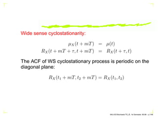
Wide sense cyclostationarity:
µX(t + mT) = µ(t)
RX(t + mT + τ, t + mT) = RX(t + τ, t)
The ACF of WS cyclostationary process is periodic on the
diagonal plane:
RX(t1 + mT, t2 + mT) = RX(t1, t2)
AKU-EE/Stochastic/HA, 1st Semester, 85-86 – p.1/46

Example:
R(t + τ, t) = E{X(t1)X(t2)} =

1, (n − 1)T ≤ t, t + τ ≤ nT
0, otherwise
R̄(τ) =
1
T
Z T
0
R(t + τ, t)dt ⇒ 0 ≤ t ≤ T
If τ 0 then RX(t + τ, t) = 1 iff τ T and t T − τ ⇒

R̄(τ) =
1
T
Z T−τ
0
1 dt = 1 −
τ
T
, 0 ≤ τ ≤ T
If τ 0 then RX(t + τ, t) = 1 iff τ −T and t T + τ ⇒
R̄(τ) =
1
T
Z T+τ
0
1 dt = 1 +
τ
T
, −T ≤ τ ≤ 0 =⇒
R̄(τ) = 1 −
|τ|
T
, |τ| ≤ T

Example:
Y (t) = X2
(t), X(t) ∼ zero-mean Gaussian of ACF RX(τ)
What is RY (τ)?
E{X2
1 X2
2 } = E{X2
1 }E{X2
2 } + 2E2
{X1X2},
this is true if
X1, X2 are jointly Gaussian. ⇒

f(X1, X2) =
exp

−0.5(X1 X2)C−1
(X1 X2)T

2π
√
∆
C =

RX(0) RX(τ)
RX(τ) RX(0)

, ∆ = det C
Using eigenvalue-eigenvector decomposition, we have:
RY (τ) = R2
X(0) + 2R2
X(τ)

Example:
The Gaussian process X(t) is an input to a hard limiter,
find the ACF of the output Y (t).
RY (τ) = E{Y (t)Y (t + τ)} ⇒ Y (t)Y (t + τ) =

1
−1
= 1 . P{X(t)X(t + τ) 0} − 1 . P{X(t)X(t + τ) 0}
X1 = X(t), X2 = X(t + τ)

If Z = X/Y then XY 0 ⇒ Z 0 and XY 0 ⇒ Z 0
f(X1, X2) =
exp

−0.5(X1 X2)C−1
(X1 X2)T

2π
√
∆
C =

RX(0) RX(τ)
RX(τ) RX(0)

, ∆ = det C

P{Z 0} = P{X1X2 0} = 1 −
Z ∞
0
Z Y Z=0
−∞
f(X1, X2)dX1dX2
+
Z 0
−∞
Z −∞
Y Z=0
f(X1, X2)dX1dX2

P{Z 0} = 0.5 +
α
π
, P{Z 0} = 0.5 −
α
π
α = arcsin

RX(τ)
RX(0)


RY (τ) =
2
π
arcsin

RX(τ)
RX(0)


In probability theory, a Lévy process, named after the
French mathematician Paul Lévy, is any continuous-time
stochastic process that has stationary independent incre-
ments. The most well-known examples are the Wiener pro-
cess and the Poisson process.

A continuous-time stochastic process assigns a random
variable Xt to each point t = 0 in time. In effect it is a
random function of t. The increments of such a process are
the differences Xs −Xt between its values at different times
s t.

To call the increments of a process independent means that
increments Xs − Xt and Xu − Xv are independent random
variables whenever the two time intervals do not overlap
and, more generally, any finite number of increments as-
signed to pairwise non-overlapping time intervals are mutu-
ally (not just pairwise) independent.

To call the increments stationary means that the probability
distribution of any increment Xs − Xt depends only on the
length s−t of the time interval; increments with equally long
time intervals are identically distributed.

In the Wiener process, the probability distribution of Xs −Xt
is normal with expected value 0 and variance s − t.

In the Poisson process, the probability distribution of Xs−Xt
is a Poisson distribution with expected value (s − t)λ, where
λ 0 is the intensity or rate of the process.

The probability distributions of the increments of any Lévy
process are infinitely divisible. There is a Lévy process for
each infinitely divisible probability distribution.

The concept of infinite divisibility arises in different ways
in philosophy, physics, economics, order theory (a branch
of mathematics), and probability theory (also a branch of
mathematics). One may speak of infinite divisibility, or the
lack thereof, of matter, space, time, money, or abstract
mathematical objects. This theory is exposed in Plato’s dia-
logue Timaeus and was also supported by Aristotle. Atom-
ism denies that matter is infinitely divisible.

To say that a probability distribution F on the real line
is infinitely divisible means that if X is any random vari-
able whose distribution is F, then for every positive integer
n there exist n independent identically distributed random
variables X1, · · · , Xn whose sum is X (those n other ran-
dom variables do not usually have the same probability dis-
tribution that X has (but do sometimes, as in the case of the
Cauchy distribution)).

The Poisson distributions, the normal distributions, and the
gamma distributions are infinitely divisible probability
distributions.
Every infinitely divisible probability distribution corresponds
in a natural way to a Lévy process, i.e., a stochastic pro-
cess Xt : t = 0 with stationary independent increments
(stationary means that for s t, the probability distribution
of Xs − Xt depends only on s − t;

independent increments means that difference is
independent of the corresponding difference on any
interval not overlapping with [t, s], and similarly for any
finite number of intervals).
This concept of infinite divisibility of probability distributions
was introduced in 1929 by Bruno de Finetti.

In any Lévy process with finite moments, the nth moment
µn(t) = E(Xn
t ) is a polynomial function of t; these functions
satisfy a binomial identity:
µn(t) =
n
X
k=0

n
k

µk(t)µn−k(t)

Wiener process, so named in honor of Norbert Wiener, is
a continuous-time Gaussian stochastic process with inde-
pendent increments used in modelling Brownian motion and
some random phenomena observed in finance. It is one of
the best-known Lévy processes.

For each positive number t, denote the value of the
process at time t by Wt. Then the process is characterized
by the following two conditions:
If 0 t s
Ws − Wt ∼ N(0, s − t)
0 ≤ t s ≤ u v ⇒ Ws − Wt and Wv − Wu are
independent RVs

The erratic motion, visible through a microscope, of small
grains suspended in a fluid. The motion results from
collisions between the grains and atoms or molecules
in the fluid. Brownian motion was first explained by
Albert Einstein, who considered it direct proof of the exis-
tence of atoms.

A geometric Brownian motion (GBM) (occasionally, expo-
nential Brownian motion) is a continuous-time stochastic
process in which the logarithm of the randomly varying
quantity follows a Brownian motion, or, perhaps more pre-
cisely, a Wiener process. It is appropriate to mathematical
modelling of some phenomena in financial markets.

A stochastic process St is said to follow a GBM if it satisfies
the following stochastic differential equation:
dSt = uStdt + vStdWt
where {Wt} is a Wiener process or Brownian motion and u
(’the percentage drift’) and v (’the percentage volatility’) are
constants.

The equation has an analytic solution:
St = S0 exp (u − v2
/2)t + vWt

for an arbitrary initial value S0.

The correctness of the solution can be verified using Itô’s
lemma. The random variable log(St/S0) is normally dis-
tributed with mean (u − v2
/2)t and variance (v.v).t, which
reflects the fact that increments of a GBM are normal rela-
tive to the current price, which is why the process has the
name ’geometric’.

In mathematics, Itô’s lemma is a theorem of stochastic cal-
culus that shows that second order differential terms of
Wiener processes become deterministic under stochastic
integration. It is somewhat analogous in stochastic calculus
to the chain rule in ordinary calculus.

Let x(t) be an Itô (or generalized Wiener) process. That is
let
dx(t) = a(x, t)dt + b(x, t)dWt
where Wt is a Wiener process, and let f(x, t) be a function
with continuous second derivatives.

Then f(x(t), t) is also an Itô process, and
df(x(t), t) =

a(x, t)
∂f
∂x
+
∂f
∂t
+
1
2
b(x, t)2 ∂2
f
∂x2

+ b(x, t)
∂f
∂x
dWt

A formal proof of the lemma requires us to take the limit of
a sequence of random variables. Expanding f(x, t) from
above in a Taylor series in x and t we have
df =
∂f
∂x
dx +
∂f
∂t
dt +
1
2
∂2
f
∂x2
dx2
+ · · ·

and substituting (adt + bdW) for dx gives
df =
∂f
∂x
(adt + bdW) +
∂f
∂t
dt +
1
2
∂2
f
∂x2
a2
dt2
+2abdtdW + b2
dW2

Reordering this to combine like differential terms, we have
df =

a
∂f
∂x
+
∂f
∂t

dt +
1
2
b2 ∂2
f
∂x2
dW2
+ b
∂f
∂x
dW + e

where e (an error term) is
ab
∂2
f
∂x2
dtdW +
1
2
a2 ∂2
f
∂x2
dt2
+ · · · .
In the limit as dt tends to 0, the dt2
and dt dW terms
disappear but the dW2
term tends to dt. The latter can be
shown if we prove that
dW2
→ E(dW2
), since E(dW2
) = dt.
The proof of this statistical property is however beyond the
scope of this course.

Substituting this dt in and reordering the terms so that the
dt and dW terms are collected, we obtain
df =

a
∂f
∂x
+
∂f
∂t
+
1
2
b2 ∂2
f
∂x2

dt + b
∂f
∂x
dW

A random walk is a formalization of the intuitive idea of tak-
ing successive steps, each in a random direction. A random
walk is a simple stochastic process.

The simplest random walk is a path constructed according
to the following rules:
There is a starting point.
The distance from one point in the path to the next is a
constant.
The direction from one point in the path to the next is
chosen at random, and no direction is more probable
than another.

Imagine now a bug walking around in the city. The city
is infinite and completely ordered, and at every corner he
chooses one of the four possible routes (including the one
he came from) with equal probability.

Formally, this is a random walk on the set of all points in the
plane with integer coordinates. Will the bug ever get back to
his home from the bar? It turns out that he will. This is the
high dimensional equivalent of the level crossing problem
discussed before.

However, the similarity stops here. In dimensions 3 and
above, this no longer holds. In other words, a drunk bird
might forever wander around, never finding its nest. The
formal terms to describe this phenomenon is that random
walk in dimensions 1 and 2 is recurrent while in dimension
3 and above it is transient. This was proved by Pólya in
1921.

The trajectory of a random walk is the collection of sites it
visited, considered as a set with disregard to when the walk
arrived at the point. In 1 dimension, the trajectory is simply
all points between the minimum height the walk achieved
and the maximum (both are, on average, on the order of
√
n).

In higher dimensions the set has interesting geometric prop-
erties. In fact, one gets a discrete fractal, that is a set
which exhibits stochastic self-similarity on large scales, but
on small scales one can observe “jugginess” resulting from
the grid on which the walk is performed.

A fractal is a geometric object which is rough or irregular on
all scales of length, and so which appears to be ’broken up’
in a radical way. Some of the best examples can be divided
into parts, each of which is similar to the original object.

Fractals are said to possess infinite detail, and some of
them have a self-similar structure that occurs at different
levels of magnification. In many cases, a fractal can be
generated by a repeating pattern, in a typically recursive
or iterative process.

A self-similar object is exactly or approximately similar to a
part of itself. A curve is said to be self-similar if, for every
piece of the curve, there is a smaller piece that is similar
to it. For instance, coastlines, are statistically self-similar:
parts of them show the same statistical properties at many
scales.

Self-similarity is a typical property of fractals. Coastlines
hypothetically can be divided into two halves, each of which
is similar to the whole.

Stochastic Processes - part 2

Recomendados

Recomendados

Mais conteúdo relacionado

Mais procurados

Mais procurados (20)

Semelhante a Stochastic Processes - part 2

Semelhante a Stochastic Processes - part 2 (20)

Último

Último (20)

Stochastic Processes - part 2