SlideShare uma empresa Scribd logo
1 de 10
Baixar para ler offline
Antunes, R., Gonzalez, V., and Walsh, K. 2015. Identification of repetitive processes at steady- and
unsteady-state: Transfer function. In: Proc. 23rd Ann. Conf. of the Int’l. Group for Lean Construction.
Perth, Australia, July 29-31, pp. 793-802, available at www.iglc.net
793 Proceedings IGLC-23, July 2015 |Perth, Australia
IDENTIFICATION OF REPETITIVE
PROCESSES AT STEADY- AND UNSTEADY-
STATE: TRANSFER FUNCTION
Ricardo Antunes1, Vicente A. González2, and Kenneth Walsh3
ABSTRACT
Projects are finite terminating endeavors with distinctive outcomes, usually, occurring
under transient conditions. Nevertheless, most estimation, planning, and scheduling
approaches overlook the dynamics of project-based systems in construction. These
approaches underestimate the influence of process repetitiveness, the variation of
learning curves and the conservation of processes’ properties. So far, estimation and
modeling approaches have enabled a comprehensive understanding of repetitive
processes in projects at steady-state. However, there has been little research to
understand and develop an integrated and explicit representation of the dynamics of
these processes in either transient, steady or unsteady conditions. This study evaluates
the transfer function in its capability of simultaneously identifying and representing
the production behavior of repetitive processes in different state conditions. The
sample data for this research comes from the construction of an offshore oil well and
describes the performance of a particular process by considering the inputs necessary
to produce the outputs. The result is a concise mathematical model that satisfactorily
reproduces the process’ behavior. Identifying suitable modeling methods, which
accurately represent the dynamic conditions of production in repetitive processes,
may provide more robust means to plan and control construction projects based on a
mathematically driven production theory.
KEYWORDS
Production, process, system identification, transfer function, system model, theory;
INTRODUCTION
Construction management practices often lack the appropriate level of ability to
handle uncertainty and complexity (McCray and Purvis, 2002; Abdelhamid, 2004)
involved in project-based systems resulting in projects failures in terms of projects
schedule and budget performance, among other measures (Mills, 2001). Traditional
scheduling approaches in construction, such as critical path method, have been
1
Ph.D. candidate, Department of Civil and Environmental Engineering - University of Auckland,
New Zealand, rsan640@aucklanduni.ac.nz
2
Senior Lecturer, Department of Civil and Environmental Engineering - University of Auckland,
New Zealand, v.gonzalez@auckland.ac.nz
3
Dean, SDSU-Georgia, San Diego State University, Tbilisi, Georgia, kwalsh@mail.sdsu.edu
Ricardo Antunes, Vicente A. González, and Kenneth Walsh
794 Proceedings IGLC-23, July 2015 |Perth, Australia
unrestrictedly used producing unfinished and erratic plans (Abdelhamid, 2004;
Bertelsen, 2003a) consequently creating distrust, and often being abandoned by those
conducting project work. Even more recent scheduling approaches, such as the ones
based on the line-of-balance method, assume that the production in construction
operates at steady-state with constant production rates (Lumsden, 1968; Arditi, et al.,
2001), where any deviation is understood as variability (Poshdar, et al., 2014).
However, “the assumption that production rates of construction projects and
processes are linear may be erroneous” (Lutz and Hijazi, 1993). Production
throughput is highly variable in construction projects (Gonzalez, Alarcon and
Molenaar, 2009), has transients (Lutz and Hijazi, 1993), occasionally is at unsteady-
state (Bernold, 1989; Walsh, et al., 2007) and frequently is nonlinear (Bertelsen,
2003b). As such, approaches that depend on constant production rates, i.e., a steady
system, possibly produce erroneous and imprecise outcomes.
The dynamics of the production system in construction is frequently overlooked
(Bertelsen, 2003b), and the transient phase is ignored (Lutz and Hijazi, 1993). The
general construction management makes no distinction between the production
dynamics and disturbance, considering both as variability (Poshdar, et al., 2014).
However, dynamics, disturbance, and variability have different meanings and action
approaches. The dynamics is an essential characteristic of any process, representing
the effects of the interaction of components in a system. Process dynamics should be
understood, managed and optimized. External factors cause disturbance, which must
be filtered, mitigated and avoided consequently reducing any impact on the process,
e.g., risk management (Antunes and Gonzalez, 2015). The understanding of these
concepts is fundamental to the development of mathematical relations and laws
suitable to the construction production system. At this time, construction adopts the
manufacturing model, dismissing the application of mathematical approaches to
model and manage its production system (Laufer, 1997; McCray and Purvis, 2002;
Bertelsen, 2003a).
Although much work has been done to date on production estimates of repetitive
processes, more studies need to be conducted to understand and develop the dynamics
of these processes. The purpose of this study is to evaluate the transfer function in its
capability of identifying and describing the dynamics of project-driven systems in
repetitive processes in construction. This topic was identified as being of importance
to point out a unique mathematical representation of project-based systems process in
transient, unsteady-, and steady-state, furthermore, overcoming a major limitation of
fixed production rates estimation approaches. The understanding of project dynamics
should improve estimation accuracy approaches and support suitable derivations of
manufacturing management practices in order to increase productivity in construction
projects. This study is a step towards the development of a mathematically driven
production theory for construction.
A SYSTEM VIEW
Mathematical models have enabled a comprehensive understanding of production
mechanisms supporting practices to improve production in manufacturing. Hopp and
Spearman (1996) committed to the comprehension of the manufacturing production
system. The system approach or system analysis was the problem-solving
methodology of choice (Hopp and Spearman, 1996). The first step of this
IDENTIFICATION OF REPETITIVE PROCESSES AT STEADY- AND UNSTEADY-STATE:
TRANSFER FUNCTION
POSTERS 795
methodology is a system view. In the system view, the problem is observed as a
system established by a set of subsystems that interact with each other. Using the
system approach, Hopp and Spearman elaborated significant laws to queue systems
and the general production in manufacturing. The conservation of material and
capacity laws (Hopp and Spearman, 1996) are particularly attractive, not only
according to their importance, but also because they explicitly state one or more
system restrictions. These laws place reliance on stable systems, with long runs and at
steady-state conditions. However, production in project-based systems, such as
construction, involves a mix of processes in steady- and unsteady-state, short and
long production runs, and different learning curves (Antunes and Gonzalez, 2015).
Hence, unless a construction process fulfills the stability and steady-state conditions,
the manufacturing model and, consequently, the laws do not accurately represent
production in construction. Alternatively, variants of manufacturing laws must be
developed to production in project-based systems that not fulfill those requirements.
In this scenario of variety, it is crucial distinguishing between project-based systems
conditions, comprehending process dynamics and its behavior.
SYSTEM IDENTIFICATION
The objective of system identification is to build mathematical models of dynamic
systems using measured data from a system (Ljung, 1998). There are several system
identification approaches to model different systems, for instance, transfer function.
The transfer function is particularly useful because it provides an algebraic
description of a system as well means to calculate parameters of the system dynamics
and stability. Nevertheless, the modeling capability of the transfer function in
construction must be evaluated and tested. In this study, the modeling approach, i.e.,
transfer function, focuses on replicating the input/output “mapping” observed in a
sample data. When the primary goal is the most accurate replication of data,
regardless of the mathematical model structure, a black-box modeling approach is
useful. Additionally, black-box modeling supports a variety of models (Bapat, 2011;
Billings, 2013), which have traditionally been practical for representing dynamic
systems. It means that at the end of the modeling, a mathematical description
represents the actual process performance rather than a structure biased by
assumptions and restrictions. Black-box modeling is a trial-and-error method, where
parameters of various models are estimated, and the output from those models is
compared to the results with the opportunity for further refinement. The resulting
models vary in complexity depending on the flexibility needed to account for both the
dynamics and any disturbance in the data. The transfer function is used in order to
show the system dynamics explicitly.
TRANSFER FUNCTION
The transfer function of a system, G, is a transformation from an input function into
an output function, capable of describing an output (or multiple outputs) by an input
(or multiple inputs) change, y(t) = G(t)⋆u(t). Although generic, the application of the
transfer function concept is restricted to systems that are represented by ordinary
differential equations (Mandal, 2006). Ordinary differential equations can represent
most dynamic systems in its entirety or at least in determined operational regions
producing accurate results (Altmannand Macdonald, 2005; Mandal, 2006). As a
Ricardo Antunes, Vicente A. González, and Kenneth Walsh
796 Proceedings IGLC-23, July 2015 |Perth, Australia
consequence, the transfer function modeling is extensively applied in the analysis and
design of systems (Ogata, 2010). A generic transfer function makes possible
representing the system dynamics by algebraic equations in the frequency domain, s.
In the frequency domain, the convolution operation transforms into an algebraic
multiplication in s, which is simpler to manipulate. Mathematically, “the transfer
function of a linear system is defined as the ratio of the Laplace transform of the
output, y(t), to the Laplace transform of the input, u(t), under the assumption that all
initial conditions are zero” (Mandal, 2006), Equation 1. Where the highest power of s
in the denominator of the transfer function is equal to n, the system is called anth-
order system.
Equation 1: Transfer function
TRANSIENT STATE, STEADY-STATE, AND UNSTEADY-STATE RESPONSE
Two parts compose a system response in the time domain, transient, and steady- or
unsteady-state. Transient is the immediate system response to an input from an
equilibrium state. After the transient state, a system response can assume a steady- or
unsteady-state. In a stable system, the output tends to a constant value when t→∞
(Mandal, 2006). When the system response enters and stays in the threshold around
the constant value the system reached the steady-state (Mandal, 2006). The time the
stable system takes to reach the steady-state is the settling time, ts. On the other hand,
if the response never reaches a final value or oscillates surpassing the threshold when
t→∞ the system is then at unsteady-state. Consequently, the system outputs at
unsteady-state vary with time during the on-time interval even induced by an
invariable input.
METHODOLOGY
A sample of 395 meters of continuous drilling was randomly selected from the
project of an offshore oil well construction, constituting the process to be modeled.
The information containing the drill ahead goal and the current process duration was
collected from operational reports and resampled to 181 samples representing the
hourly process behavior when commanded by the input, establishing a system. Next,
the estimation of a transfer function was used for the determination of a model that
represents the dynamics of the system-based process. The estimation uses nine
partitions of the dataset creating models based on different data sizes. The best model
from each of the nine partitions presenting the lowest estimation unfitness value were
selected and cross-validated by the remaining data. Later, the system response of the
best model was analyzed.
CASE STUDY: DRILLING AS A SYSTEM
The subject of this study is the drilling process on a particular offshore well
construction project in Brazilian pre-salt. This process was chosen given its high level
of repetitiveness. The vertical dimension of repetitiveness is the repetition of the
process in the project, i.e., the drilling occurs more than one time in the construction
of a well. The horizontal dimension is the repetition of the process in different
IDENTIFICATION OF REPETITIVE PROCESSES AT STEADY- AND UNSTEADY-STATE:
TRANSFER FUNCTION
POSTERS 797
projects, i.e., the drilling occurs on every well construction project. Such degree of
repetitiveness eases comparison and data validation because a repetitive process tends
to present patterns in smaller data portions. The case documentation provides details
about inputs, outputs and brief explanations of the process parameters. Nonetheless,
the documentation does not include any mathematical representation of the processes
other than the drilling parameters and other activities performed while drilling, which
constitute subsystems. For instance, the work instructions to drill a segment of 28
meters on seabed:
 Drill ahead 8 1/2" hole from 3684 m to 3712 m with 480 gpm, 1850 psi, 15-
25k WOB, 120 rpm, 15-20 kft.lbs torq. Perform surveys and downlinks as per
directional driller instructions. Pump 15 bbl fine pill and 50 bbl hi-vis pill
every two stand as per mud engineer instructions.
The primary input, ‘drill ahead from 3684 m to 3712 m’, and the parameters, such as
torque and rpm, directly affect the drilling process. However, the system view unifies
the different parts of the system, i.e., the subsystems, into an effectual unit using a
holistic perspective. The holistic perspective allows the creation of a system driven by
a primary input while all others variables interact as subsystems of the main system.
To fully establish a system, an input has to be applied to the process in order
produce an output. Accordingly, the input, u(t), consists of a drilling ahead depth
goal, e.g., 3712 meters, that is applied to the drilling process, producing the output,
y(t), that is the actual depth, in meters. In the process, G(t), the drilling crew responds
to the drilling ahead goal by drilling and performing related tasks, which increases the
actual well depth over time until reaching the drilling depth goal. Then, a new drill
ahead goal is set, and the process performs the cycle. The sample data corresponds
with a well depth increase from 3305 to 3700 meters at a variable rate based on
operational choices. The 181 samples represent the hourly input and process behavior
response, i.e., output. The input and output data are cumulative due to physical
restrictions. In other words, it is impossible to drill from 3435 meters without prior
drilling from the seabed at 924 meters from water level to 3435 meters in the hole.
Consequently the drill ahead goal as well as the actual depth values are always greater
than the previous values. Figure 1 displays the general system representation of the
process with its measured input and output, drill ahead goal and actual depth
respectively. Two criteria guided the choice of drilling goal as input. The first
criterion is that the drill ahead goal is the primarily directive to achieve the objective
of the project, setting the peace to build the well. The drill ahead goal is an adaptive
plan in which the team has to examine the current conditions of the well and
determine the best drill ahead goal. It relies on guidelines and procedures but in the
end its a human decision. The second criterionis that this particular arrangement
illustrates the number of items arriving in a queuing system at time t. Additionally,
the output represents the number of items departing in the queuing system at time t.
Such input-output arrangement is instrumental to adapt manufacturing-based models
such as the Little’s Law (Little, 1961) to construction in further research.
Ricardo Antunes, Vicente A. González, and Kenneth Walsh
798 Proceedings IGLC-23, July 2015 |Perth, Australia
Figure 1. System representation of the case study
INITIAL MODELING APPROACH
A simple model is attempted initially before progressing to more complex structures
until reaching the required model accuracy. Simpler models are easier to interpret, a
desired feature in this study. However, if that model unsatisfactorily simulates the
measured data, it may be necessary to use more complex models. The simpler system
identification approach is the transfer function. Hence, transfer function might be a
good starting point in order to identify, model and understand the behavior of a
system. The sample data was partitioned in nine combinations representing nine
stages in time, as shown in Figure 1. The first partition is at the 20th hour. Therefore,
the data from zero to 20 hours was used as estimation data for G1, and from 21 to 181
hours as the validation data. The second partition happens at 40 hours mark. In the
same way, the estimation for G2 is composed of the data from zero to 40 hours mark,
and the validation is from the 41st to the 181st hour. This pattern repeats until the
180-time stamp. At this partition, almost the whole sample constitutes the estimation
data, and only one sample is left for validation of G9. The model from this partition,
G9, merely fits the estimation data once there is virtually no data that could be used to
validate the model. Based on black-box trial-and-error approach, the model
parameters of the transfer function of first-order (Ogata, 2010) were generated for
each partition using the iterative prediction-error minimization algorithm (Ljung,
2010) from MATLAB’s System Identification Toolbox. A first-order transfer
function eases the model interpretability.
MODEL DEVELOPMENT
Three transfer functions, which showed the lowest unfitness values, calculated by
100% – normalized root mean square (NRMSE) (Armstrong and Collopy, 1992;
Ljung, 2010), were selected for each of the nine data partitions, constituting the best
models. A perfect fit corresponds to zero meaning that the simulated or predicted
model output is exactly the same as the measured data.
MODEL QUALITY ASSESSMENT
The initial models were later refined using the prediction-error minimization
algorithm (Ljung, 1998). After refinement, the models that achieved the lowest
unfitness values to each estimation data partition that they derived from were then
validated using the remaining data of their partition. Figure 2 shows the quality
measurements of the best models for each partition. The quality measurements are the
percentage of validation and estimation data unfitness, Akaike's Final Prediction
Error (FPE) (Jones, 1975), loss function (Berger, 1985) and mean squared normalized
error performance function (MSE) (Poli and Cirillo, 1993). The quality measurements
IDENTIFICATION OF REPETITIVE PROCESSES AT STEADY- AND UNSTEADY-STATE:
TRANSFER FUNCTION
POSTERS 799
are represented in the graph by ‘Val unfit’, ‘Est unfit’, FPE, ‘Loss Fcn’, and MSE
respectively. Although, the model choice in this study is not mathematically based on
FPE, loss function and MSE their values were calculated and shown providing an
extra measurement of model quality. A variety of measurements is useful for
comparing different models as well as comparing the models with different modeling
approaches. Differently from the models one to seven, the models for the segments
eight and nine present high unfit levels to their validation segments, 72,64% and
impossible to calculate, respectively. For G8, the input-output relation of the
validation data, shown in the segment eight to nine in Figure 2, is extremely distinct
from the data used in the estimation, segment one to eight. For G9, there is only one
sample remaining to validate the model. Hence, the model
G9(s) = 0.6646 / (s + 0.6687) corresponds to the structure that better reproduces the
sample data with about 93% fitness. Accordingly, G9 is used later to demonstrated the
step response.
Figure 2. Quality comparison of the models
Despite the model G9 has the lowest unfitted data, ‘Est unfit’, almost the whole
sample data was used to estimateG9. Hence, G9 already ‘knows’the data sample and
for this reason cannot be used as a predictor. In order to illustrate the prediction
accuracy of the models, the model with the largest ‘unknown’ data, i.e., G1 is used.
Figure 3 shows the comparison of the measured data and model G1(t), result of
inverse Laplace Transform ofG1(s) = 0.4193 / (s + 0.4103);the solid line is the
measured output and the dashed line the model response with 9.5% unfitness. The
transfer function G1(t), can represent the process input-output relationship with
sufficient precision. Furthermore, the model is estimated at an early stage, around the
initial 10% duration, independently of any previous process knowledge.
Figure 3. Comparison between the G1 response and measured data
STEP RESPONSE
Figure 4(a) shows the step response for the model G9. The model reaches steady-state
about the sixth hour for a threshold of absolute two percent about the final value. The
step amplitude used as input, 2.06, is the average drilling goal ahead. The system
responds to this input reaching and staying steady at the output peak, yp = 2.05, about
0 20 40 60 80 100 120 140 160 180
3300
3350
3400
3450
3500
3550
3600
3650
3700
y (t) = 0.4193e
−0.4103 t
* u(t)
Time (hours)
Actualdepth(meters)
Estimation Prediction
Actual output
Model response
Ricardo Antunes, Vicente A. González, and Kenneth Walsh
800 Proceedings IGLC-23, July 2015 |Perth, Australia
the 16th hour, tp. In this case, the steady-state value is the peak value because it is the
value that the system tends to when t→∞ (Mandal, 2006). The average drilling rate
from the measured output data is 2.1 meters per hour approximately the model output
at steady-state, with a three percent error. Consequently, the model represents the
system at steady-state. Although, the transient response stands for a significant part of
the system dynamics. The system has a transient response every time it starts or stops.
Although it stays at the transient state when it need small corrections, as, for instance,
to fit a casing pipe to secure the well. In this case, the system also has inputs as small
as one. For this input, the average response of the system is 0.55 meters per hour. In
order to assess the system transient response, a unitary step unit was introduced to the
system producing the system response, as shown in Figure 4(b). The average response
for the unitary input is achieved around one hour by the system indicating that the
system is performing in the transient state.
Figure 4. (a) 2.06 step response (b) Unit step response
CONCLUSIONS
The results of the model’s accuracy were explicit. The models were consistent with
the modeling approach and methodology. The valid transfer functions obtained
reliablydescribed the process behavior and presented evidence of their accuracy using
a range of model quality measurements. These findings thus lend support to the use of
transfer function as a valid model approach and analytical technique in order to
describe the dynamic conditions of production in repetitive processes in projects.
Accounting for transient responses, transfer function fulfills a gap left by network
scheduling and queueing theory as well as linear and dynamic programming, which
ignore the transient stage and assume that the process is at steady-state. Moreover, a
transfer functions may act as a multi-level management tool. Because transfer
functions provide an output function from an input function, they enable the creation
of accurate plans rather than single actions and a throughput function, instead of a
system position. Transfer functions may be used by site managers as a process
descriptor to monitor and control low-level activities, as shown in Figure 3. Dynamic
and accurate plans that respond to actual inputs can regain the trust of those
conducting the project work on planning and scheduling. Moreover, the model
simulation may be used in a means-ends analysis determining the best solution to a
construction process, which frequently requires the optimization of resources to the
detriment of shorter duration. In other words, managers may use the model adjusting
the drill ahead goal plan until attaining the defined goal, supporting managers’
IDENTIFICATION OF REPETITIVE PROCESSES AT STEADY- AND UNSTEADY-STATE:
TRANSFER FUNCTION
POSTERS 801
decision-making process. Once the managers are satisfied with both the drill ahead
goal plan and the system’s outcome, the plan is executed. A transfer function may
also be applied to represent higher levels, providing project managers a holistic view.
Reliance on this method must be tempered, however because the case does not
represent the general conditions of repetitive process in construction. There is a
variety of construction processes that happen in different states, production runs, and
different learning curves creating unique process’ characteristics. For instance, this
study presents the analysis of system’s transient and steady-state response, but not
unsteady-state because the case scenario does not have this characteristic. Although
the model can be reused in similar processes as an initial model, a limitation places on
the existence of the process’ input-output data. It means that the model accuracy
cannot be evaluated until some data has been produced. Finally, the study explores
several concepts that are unfamiliar to general construction managers at this point
restricting its audience. Nevertheless, the search for and the aggregation of
knowledge and expertise from different disciplines and technical fields constitutes the
foremost forces driving the evolution in managerial sciences.
FUTURE OUTCOMES
Different system identification approaches can write equations for practically any
process. However, only after extensive research about the dynamic conditions of
production in project-driven systems the lack of knowledge about the transient and
unsteady-state responses can be replaced by explanatory and mathematical laws to
production in projects. In a further horizon, processes transient and unsteady-state
will be understood and managed to generate an optimum process outcome. Being it
reducing the transient time, and faster-moving processes to steady-state or applying
unsteady-state processing techniques producing an average output above steady-state
levels and then creating high-performance processes.
REFERENCES
Abdelhamid, T. S. 2004. The self-destruction and renewal of lean construction
theory: A prediction from Boyd-s theory. In: Proc. 12th
Ann. Conf. of the Int’l.
Group for Lean Construction. Helsingør, Denmark, Aug. 3-5.
Altmann, W. and Macdonald, D., 2005. Practical Process Control for Engineers and
Technicians. Burlington, MA: Elsevier.
Antunes, R. and Gonzalez, V., 2015. A production model for construction: A
theoretical framework. Buildings, 5(1), pp. 209-228.
Arditi, D., Tokdemir, O. B. and Suh, K., 2001. Effect of learning on line-of-balance
scheduling. International Journal of Project Management, 19(5), pp. 265-277.
Armstrong, J. S. and Collopy, F., 1992. Error measures for generalizing about
forecasting methods: Empirical comparisons. International Journal of
Forecasting, 8(1), pp. 69-80.
Bapat, R. B., 2011. Linear Algebra and Linear Models. 3rd ed. New Delhi: Springer.
Berger, J. O., 1985. Statistical Decision Theory and Bayesian Analysis. Springer
Series in Statistics. New York: Springer.
Bernold, L. E., 1989. Simulation of Nonsteady Construction Processes. Journal of
Construction Engineering and Management, 115(2), pp. 163-178.
Ricardo Antunes, Vicente A. González, and Kenneth Walsh
802 Proceedings IGLC-23, July 2015 |Perth, Australia
Bertelsen, S. 2003a. Complexity- Construction in a New Perspective. In: Proc.
11th
Ann. Conf. of the Int’l. Group for Lean Construction. Blacksburg, VA, Jul. 21-
24.
Bertelsen, S. 2003b. Construction as a Complex System. In: Proc. 11th
Ann. Conf. of
the Int’l. Group for Lean Construction. Blacksburg, VA, Jul. 21-24
Billings, S. A., 2013. Nonlinear System Identification Narmax Methods in the Time,
Frequency, and Spatio-Temporal Domains. West Sussex: John Wiley & Sons.
Garnier, H. and Wang L. Eds. 2008. Identification of Continuous-time Models from
Sampled Data. London: Springer-Verlag.
González, V., Alarcón, L. F. and Molenaar, K., 2009. Multiobjective Design of
Work-In-Process Buffer for Scheduling Repetitive Building Projects. Automation
in Construction, 18(2), pp. 95-108.
Hopp, W. J. and Spearman, M. L., 1996. Factory Physics: Foundations of
Manufacturing Management. 2nd ed. New York: Irwin McGraw-Hill.
Jones, R. H., 1975. Fitting Auto regressions. Journal of the American Statistical
Association, 70(351), pp. 590-592.
Laufer, A., 1997. Simultaneous management: Managing projects in a dynamic
environment. New York: American Management Association.
Little, J. D. C., 1961. A Proof for the Queuing Formula: L= λ W. Operations
Research, 9(3), pp. 383-387.
Ljung, L., 1998. System Identification: Theory for the User. Upper Saddle River, NJ:
Pearson Education.
Ljung, L., 2010. System Identification Toolbox 7. Reference. Natick, MA:
Mathworks.
Lumsden, P. 1968. The Line-of-balance method. Oxford: Pergamon Press, Industrial
Training Division.
Lutz, J. D. and Hijazi, A., 1993. Planning repetitive construction: Current practice.
Construction Management and Economics, 11(2), pp.99-110.
Mandal, A. K. 2006. Introduction to Control Engineering: Modeling, Analysis and
Design. New Delhi: New Age International Publishers.
McCray, G. E. and Purvis, R. L., 2002. Project management under uncertainty: the
impact of heuristics and biases. Project Management Journal, 33(1), pp. 49-57.
Mills, A., 2001. A systematic approach to risk management for construction.
Structural Survey, 19(5), pp. 245-252.
Ogata, K., 2010. Modern Control Engineering. 5th ed. Upper Saddle River, NJ:
Prentice Hall.
Poli, A. A. and Cirillo, M. C., 1993. On the use of the normalized mean square error
in evaluating dispersion model performance. Atmospheric Environment. Part A.
General Topics, 27(15), 2427-2434.
Poshdar, M., González, V. A., Raftery, G. and Orozco, F., 2014. Characterization of
Process Variability in Construction. Journal of Construction Engineering and
Management, 140, (11) 05014009.
Walsh, K. D., Sawhney, A. and Bashford, H. H., 2007. Production Equations for
Unsteady-State Construction Processes. Journal of Construction Engineering and
Management, 133(3), pp. 245-261.

Mais conteúdo relacionado

Semelhante a Identification of repetitive processes at steady- and unsteady-state: Transfer function

**Exploring and Assessing Project Complexity-Dao;17.pdf
**Exploring and Assessing Project Complexity-Dao;17.pdf**Exploring and Assessing Project Complexity-Dao;17.pdf
**Exploring and Assessing Project Complexity-Dao;17.pdfDépartement de finance
 
10.1.1.64.430
10.1.1.64.43010.1.1.64.430
10.1.1.64.430ankoos
 
Lean manufacturing context_practice_bundles_and_pe
Lean manufacturing context_practice_bundles_and_peLean manufacturing context_practice_bundles_and_pe
Lean manufacturing context_practice_bundles_and_peAngela Castillo
 
Statistical Data Analysis.docx
Statistical Data Analysis.docxStatistical Data Analysis.docx
Statistical Data Analysis.docxAzrul Fazwan
 
A learning based transportation oriented simulation system
A learning based transportation oriented simulation systemA learning based transportation oriented simulation system
A learning based transportation oriented simulation systemWolfsbane_John
 
Applicability of heuristic approach in planning and scheduling project
Applicability of heuristic approach in planning and scheduling projectApplicability of heuristic approach in planning and scheduling project
Applicability of heuristic approach in planning and scheduling projectAlexander Decker
 
Stochastic behavior analysis of complex repairable industrial systems
Stochastic behavior analysis of complex repairable industrial systemsStochastic behavior analysis of complex repairable industrial systems
Stochastic behavior analysis of complex repairable industrial systemsISA Interchange
 
IRJET- Review on Scheduling using Dependency Structure Matrix
IRJET-  	  Review on Scheduling using Dependency Structure MatrixIRJET-  	  Review on Scheduling using Dependency Structure Matrix
IRJET- Review on Scheduling using Dependency Structure MatrixIRJET Journal
 
Impact of Information Technology Change in the Operations System
Impact of Information Technology Change in the Operations SystemImpact of Information Technology Change in the Operations System
Impact of Information Technology Change in the Operations SystemBaker Khader Abdallah, PMP
 
Evaluation of Process Capability Using Fuzzy Inference System
Evaluation of Process Capability Using Fuzzy Inference SystemEvaluation of Process Capability Using Fuzzy Inference System
Evaluation of Process Capability Using Fuzzy Inference SystemIOSR Journals
 
Optimization of Assembly Line and Plant Layout in a Mass Production Industry...
	Optimization of Assembly Line and Plant Layout in a Mass Production Industry...	Optimization of Assembly Line and Plant Layout in a Mass Production Industry...
Optimization of Assembly Line and Plant Layout in a Mass Production Industry...inventionjournals
 
A review of advanced linear repetitive scheduling methods and techniques
A review of advanced linear repetitive scheduling methods and techniquesA review of advanced linear repetitive scheduling methods and techniques
A review of advanced linear repetitive scheduling methods and techniquesAsadullah Malik
 
Is robustness really robust? how different definitions of robustness impact d...
Is robustness really robust? how different definitions of robustness impact d...Is robustness really robust? how different definitions of robustness impact d...
Is robustness really robust? how different definitions of robustness impact d...Environmental Intelligence Lab
 
New Product Development as a Complex Adaptive System of Decisions
New Product Development as a Complex Adaptive System of DecisionsNew Product Development as a Complex Adaptive System of Decisions
New Product Development as a Complex Adaptive System of DecisionsIan McCarthy
 
Using fuzzy set qualitative comparative analysis to measure contract rules in...
Using fuzzy set qualitative comparative analysis to measure contract rules in...Using fuzzy set qualitative comparative analysis to measure contract rules in...
Using fuzzy set qualitative comparative analysis to measure contract rules in...Maria Kapsali (PhD)
 

Semelhante a Identification of repetitive processes at steady- and unsteady-state: Transfer function (20)

**Exploring and Assessing Project Complexity-Dao;17.pdf
**Exploring and Assessing Project Complexity-Dao;17.pdf**Exploring and Assessing Project Complexity-Dao;17.pdf
**Exploring and Assessing Project Complexity-Dao;17.pdf
 
10.1.1.64.430
10.1.1.64.43010.1.1.64.430
10.1.1.64.430
 
Lean manufacturing context_practice_bundles_and_pe
Lean manufacturing context_practice_bundles_and_peLean manufacturing context_practice_bundles_and_pe
Lean manufacturing context_practice_bundles_and_pe
 
Jw3517111716
Jw3517111716Jw3517111716
Jw3517111716
 
Kanban
KanbanKanban
Kanban
 
Statistical Data Analysis.docx
Statistical Data Analysis.docxStatistical Data Analysis.docx
Statistical Data Analysis.docx
 
A learning based transportation oriented simulation system
A learning based transportation oriented simulation systemA learning based transportation oriented simulation system
A learning based transportation oriented simulation system
 
Work Package 3
Work Package 3Work Package 3
Work Package 3
 
Applicability of heuristic approach in planning and scheduling project
Applicability of heuristic approach in planning and scheduling projectApplicability of heuristic approach in planning and scheduling project
Applicability of heuristic approach in planning and scheduling project
 
Stochastic behavior analysis of complex repairable industrial systems
Stochastic behavior analysis of complex repairable industrial systemsStochastic behavior analysis of complex repairable industrial systems
Stochastic behavior analysis of complex repairable industrial systems
 
IRJET- Review on Scheduling using Dependency Structure Matrix
IRJET-  	  Review on Scheduling using Dependency Structure MatrixIRJET-  	  Review on Scheduling using Dependency Structure Matrix
IRJET- Review on Scheduling using Dependency Structure Matrix
 
Impact of Information Technology Change in the Operations System
Impact of Information Technology Change in the Operations SystemImpact of Information Technology Change in the Operations System
Impact of Information Technology Change in the Operations System
 
Evaluation of Process Capability Using Fuzzy Inference System
Evaluation of Process Capability Using Fuzzy Inference SystemEvaluation of Process Capability Using Fuzzy Inference System
Evaluation of Process Capability Using Fuzzy Inference System
 
Optimization of Assembly Line and Plant Layout in a Mass Production Industry...
	Optimization of Assembly Line and Plant Layout in a Mass Production Industry...	Optimization of Assembly Line and Plant Layout in a Mass Production Industry...
Optimization of Assembly Line and Plant Layout in a Mass Production Industry...
 
ONE HIDDEN LAYER ANFIS MODEL FOR OOS DEVELOPMENT EFFORT ESTIMATION
ONE HIDDEN LAYER ANFIS MODEL FOR OOS DEVELOPMENT EFFORT ESTIMATIONONE HIDDEN LAYER ANFIS MODEL FOR OOS DEVELOPMENT EFFORT ESTIMATION
ONE HIDDEN LAYER ANFIS MODEL FOR OOS DEVELOPMENT EFFORT ESTIMATION
 
A review of advanced linear repetitive scheduling methods and techniques
A review of advanced linear repetitive scheduling methods and techniquesA review of advanced linear repetitive scheduling methods and techniques
A review of advanced linear repetitive scheduling methods and techniques
 
Cv miguel
Cv miguelCv miguel
Cv miguel
 
Is robustness really robust? how different definitions of robustness impact d...
Is robustness really robust? how different definitions of robustness impact d...Is robustness really robust? how different definitions of robustness impact d...
Is robustness really robust? how different definitions of robustness impact d...
 
New Product Development as a Complex Adaptive System of Decisions
New Product Development as a Complex Adaptive System of DecisionsNew Product Development as a Complex Adaptive System of Decisions
New Product Development as a Complex Adaptive System of Decisions
 
Using fuzzy set qualitative comparative analysis to measure contract rules in...
Using fuzzy set qualitative comparative analysis to measure contract rules in...Using fuzzy set qualitative comparative analysis to measure contract rules in...
Using fuzzy set qualitative comparative analysis to measure contract rules in...
 

Mais de Ricardo Magno Antunes

Envision of an Integrated Information System for Projectdriven Production in ...
Envision of an Integrated Information System for Projectdriven Production in ...Envision of an Integrated Information System for Projectdriven Production in ...
Envision of an Integrated Information System for Projectdriven Production in ...Ricardo Magno Antunes
 
Dynamics of project-driven systems A production model for repetitive processe...
Dynamics of project-driven systems A production model for repetitive processe...Dynamics of project-driven systems A production model for repetitive processe...
Dynamics of project-driven systems A production model for repetitive processe...Ricardo Magno Antunes
 
Quicker reaction, lower variability: The effect of transient time in flow var...
Quicker reaction, lower variability: The effect of transient time in flow var...Quicker reaction, lower variability: The effect of transient time in flow var...
Quicker reaction, lower variability: The effect of transient time in flow var...Ricardo Magno Antunes
 
A Production Model for Construction: A Theoretical Framework
A Production Model for Construction: A Theoretical FrameworkA Production Model for Construction: A Theoretical Framework
A Production Model for Construction: A Theoretical FrameworkRicardo Magno Antunes
 
Building a Better NZ conference 2014
Building a Better NZ conference 2014Building a Better NZ conference 2014
Building a Better NZ conference 2014Ricardo Magno Antunes
 
Envoiremental Concerns in Right-of-Way - An International Symposium Series RO...
Envoiremental Concerns in Right-of-Way - An International Symposium Series RO...Envoiremental Concerns in Right-of-Way - An International Symposium Series RO...
Envoiremental Concerns in Right-of-Way - An International Symposium Series RO...Ricardo Magno Antunes
 
Automação de Processos e Serviços - Aula05
Automação de Processos e Serviços - Aula05Automação de Processos e Serviços - Aula05
Automação de Processos e Serviços - Aula05Ricardo Magno Antunes
 
Automação de Processos e Serviços - Aula03
Automação de Processos e Serviços - Aula03Automação de Processos e Serviços - Aula03
Automação de Processos e Serviços - Aula03Ricardo Magno Antunes
 
Automação de Processos e Serviços - Aula02
Automação de Processos e Serviços - Aula02Automação de Processos e Serviços - Aula02
Automação de Processos e Serviços - Aula02Ricardo Magno Antunes
 
Automação de Processos e Serviços - Aula01
Automação de Processos e Serviços - Aula01Automação de Processos e Serviços - Aula01
Automação de Processos e Serviços - Aula01Ricardo Magno Antunes
 
Automação de Processos e Serviços - Aula04
Automação de Processos e Serviços - Aula04Automação de Processos e Serviços - Aula04
Automação de Processos e Serviços - Aula04Ricardo Magno Antunes
 
COST BENEFIT ANALYSIS OF URBAN TREE MANAGEMENT IN GOIÂNIA
COST BENEFIT ANALYSIS OF  URBAN TREE MANAGEMENT IN GOIÂNIA COST BENEFIT ANALYSIS OF  URBAN TREE MANAGEMENT IN GOIÂNIA
COST BENEFIT ANALYSIS OF URBAN TREE MANAGEMENT IN GOIÂNIA Ricardo Magno Antunes
 
COST BENEFIT ANALYSIS OF URBAN TREE MANAGEMENT IN GOIÂNIA
COST BENEFIT ANALYSIS OF  URBAN TREE MANAGEMENT IN GOIÂNIA COST BENEFIT ANALYSIS OF  URBAN TREE MANAGEMENT IN GOIÂNIA
COST BENEFIT ANALYSIS OF URBAN TREE MANAGEMENT IN GOIÂNIA Ricardo Magno Antunes
 

Mais de Ricardo Magno Antunes (13)

Envision of an Integrated Information System for Projectdriven Production in ...
Envision of an Integrated Information System for Projectdriven Production in ...Envision of an Integrated Information System for Projectdriven Production in ...
Envision of an Integrated Information System for Projectdriven Production in ...
 
Dynamics of project-driven systems A production model for repetitive processe...
Dynamics of project-driven systems A production model for repetitive processe...Dynamics of project-driven systems A production model for repetitive processe...
Dynamics of project-driven systems A production model for repetitive processe...
 
Quicker reaction, lower variability: The effect of transient time in flow var...
Quicker reaction, lower variability: The effect of transient time in flow var...Quicker reaction, lower variability: The effect of transient time in flow var...
Quicker reaction, lower variability: The effect of transient time in flow var...
 
A Production Model for Construction: A Theoretical Framework
A Production Model for Construction: A Theoretical FrameworkA Production Model for Construction: A Theoretical Framework
A Production Model for Construction: A Theoretical Framework
 
Building a Better NZ conference 2014
Building a Better NZ conference 2014Building a Better NZ conference 2014
Building a Better NZ conference 2014
 
Envoiremental Concerns in Right-of-Way - An International Symposium Series RO...
Envoiremental Concerns in Right-of-Way - An International Symposium Series RO...Envoiremental Concerns in Right-of-Way - An International Symposium Series RO...
Envoiremental Concerns in Right-of-Way - An International Symposium Series RO...
 
Automação de Processos e Serviços - Aula05
Automação de Processos e Serviços - Aula05Automação de Processos e Serviços - Aula05
Automação de Processos e Serviços - Aula05
 
Automação de Processos e Serviços - Aula03
Automação de Processos e Serviços - Aula03Automação de Processos e Serviços - Aula03
Automação de Processos e Serviços - Aula03
 
Automação de Processos e Serviços - Aula02
Automação de Processos e Serviços - Aula02Automação de Processos e Serviços - Aula02
Automação de Processos e Serviços - Aula02
 
Automação de Processos e Serviços - Aula01
Automação de Processos e Serviços - Aula01Automação de Processos e Serviços - Aula01
Automação de Processos e Serviços - Aula01
 
Automação de Processos e Serviços - Aula04
Automação de Processos e Serviços - Aula04Automação de Processos e Serviços - Aula04
Automação de Processos e Serviços - Aula04
 
COST BENEFIT ANALYSIS OF URBAN TREE MANAGEMENT IN GOIÂNIA
COST BENEFIT ANALYSIS OF  URBAN TREE MANAGEMENT IN GOIÂNIA COST BENEFIT ANALYSIS OF  URBAN TREE MANAGEMENT IN GOIÂNIA
COST BENEFIT ANALYSIS OF URBAN TREE MANAGEMENT IN GOIÂNIA
 
COST BENEFIT ANALYSIS OF URBAN TREE MANAGEMENT IN GOIÂNIA
COST BENEFIT ANALYSIS OF  URBAN TREE MANAGEMENT IN GOIÂNIA COST BENEFIT ANALYSIS OF  URBAN TREE MANAGEMENT IN GOIÂNIA
COST BENEFIT ANALYSIS OF URBAN TREE MANAGEMENT IN GOIÂNIA
 

Último

Call Now Pooja Mehta : 7738631006 Door Step Call Girls Rate 100% Satisfactio...
Call Now Pooja Mehta :  7738631006 Door Step Call Girls Rate 100% Satisfactio...Call Now Pooja Mehta :  7738631006 Door Step Call Girls Rate 100% Satisfactio...
Call Now Pooja Mehta : 7738631006 Door Step Call Girls Rate 100% Satisfactio...Pooja Nehwal
 
Call now : 9892124323 Nalasopara Beautiful Call Girls Vasai virar Best Call G...
Call now : 9892124323 Nalasopara Beautiful Call Girls Vasai virar Best Call G...Call now : 9892124323 Nalasopara Beautiful Call Girls Vasai virar Best Call G...
Call now : 9892124323 Nalasopara Beautiful Call Girls Vasai virar Best Call G...Pooja Nehwal
 
internal analysis on strategic management
internal analysis on strategic managementinternal analysis on strategic management
internal analysis on strategic managementharfimakarim
 
Reviewing and summarization of university ranking system to.pptx
Reviewing and summarization of university ranking system  to.pptxReviewing and summarization of university ranking system  to.pptx
Reviewing and summarization of university ranking system to.pptxAss.Prof. Dr. Mogeeb Mosleh
 
Dealing with Poor Performance - get the full picture from 3C Performance Mana...
Dealing with Poor Performance - get the full picture from 3C Performance Mana...Dealing with Poor Performance - get the full picture from 3C Performance Mana...
Dealing with Poor Performance - get the full picture from 3C Performance Mana...Hedda Bird
 
BDSM⚡Call Girls in Sector 99 Noida Escorts >༒8448380779 Escort Service
BDSM⚡Call Girls in Sector 99 Noida Escorts >༒8448380779 Escort ServiceBDSM⚡Call Girls in Sector 99 Noida Escorts >༒8448380779 Escort Service
BDSM⚡Call Girls in Sector 99 Noida Escorts >༒8448380779 Escort ServiceDelhi Call girls
 
Construction Project Management | Coursera 2024
Construction Project Management | Coursera 2024Construction Project Management | Coursera 2024
Construction Project Management | Coursera 2024Alex Marques
 
GENUINE Babe,Call Girls IN Baderpur Delhi | +91-8377087607
GENUINE Babe,Call Girls IN Baderpur  Delhi | +91-8377087607GENUINE Babe,Call Girls IN Baderpur  Delhi | +91-8377087607
GENUINE Babe,Call Girls IN Baderpur Delhi | +91-8377087607dollysharma2066
 
Agile Coaching Change Management Framework.pptx
Agile Coaching Change Management Framework.pptxAgile Coaching Change Management Framework.pptx
Agile Coaching Change Management Framework.pptxalinstan901
 

Último (20)

Intro_University_Ranking_Introduction.pptx
Intro_University_Ranking_Introduction.pptxIntro_University_Ranking_Introduction.pptx
Intro_University_Ranking_Introduction.pptx
 
Call Now Pooja Mehta : 7738631006 Door Step Call Girls Rate 100% Satisfactio...
Call Now Pooja Mehta :  7738631006 Door Step Call Girls Rate 100% Satisfactio...Call Now Pooja Mehta :  7738631006 Door Step Call Girls Rate 100% Satisfactio...
Call Now Pooja Mehta : 7738631006 Door Step Call Girls Rate 100% Satisfactio...
 
Call now : 9892124323 Nalasopara Beautiful Call Girls Vasai virar Best Call G...
Call now : 9892124323 Nalasopara Beautiful Call Girls Vasai virar Best Call G...Call now : 9892124323 Nalasopara Beautiful Call Girls Vasai virar Best Call G...
Call now : 9892124323 Nalasopara Beautiful Call Girls Vasai virar Best Call G...
 
Disrupt or be Disrupted - Kirk Vallis.pdf
Disrupt or be Disrupted - Kirk Vallis.pdfDisrupt or be Disrupted - Kirk Vallis.pdf
Disrupt or be Disrupted - Kirk Vallis.pdf
 
LoveLocalGov - Chris Twigg, Inner Circle
LoveLocalGov - Chris Twigg, Inner CircleLoveLocalGov - Chris Twigg, Inner Circle
LoveLocalGov - Chris Twigg, Inner Circle
 
internal analysis on strategic management
internal analysis on strategic managementinternal analysis on strategic management
internal analysis on strategic management
 
Becoming an Inclusive Leader - Bernadette Thompson
Becoming an Inclusive Leader - Bernadette ThompsonBecoming an Inclusive Leader - Bernadette Thompson
Becoming an Inclusive Leader - Bernadette Thompson
 
Imagine - HR; are handling the 'bad banter' - Stella Chandler.pdf
Imagine - HR; are handling the 'bad banter' - Stella Chandler.pdfImagine - HR; are handling the 'bad banter' - Stella Chandler.pdf
Imagine - HR; are handling the 'bad banter' - Stella Chandler.pdf
 
Imagine - Creating Healthy Workplaces - Anthony Montgomery.pdf
Imagine - Creating Healthy Workplaces - Anthony Montgomery.pdfImagine - Creating Healthy Workplaces - Anthony Montgomery.pdf
Imagine - Creating Healthy Workplaces - Anthony Montgomery.pdf
 
Reviewing and summarization of university ranking system to.pptx
Reviewing and summarization of university ranking system  to.pptxReviewing and summarization of university ranking system  to.pptx
Reviewing and summarization of university ranking system to.pptx
 
Discover -CQ Master Class - Rikita Wadhwa.pdf
Discover -CQ Master Class - Rikita Wadhwa.pdfDiscover -CQ Master Class - Rikita Wadhwa.pdf
Discover -CQ Master Class - Rikita Wadhwa.pdf
 
Empowering Local Government Frontline Services - Mo Baines.pdf
Empowering Local Government Frontline Services - Mo Baines.pdfEmpowering Local Government Frontline Services - Mo Baines.pdf
Empowering Local Government Frontline Services - Mo Baines.pdf
 
Dealing with Poor Performance - get the full picture from 3C Performance Mana...
Dealing with Poor Performance - get the full picture from 3C Performance Mana...Dealing with Poor Performance - get the full picture from 3C Performance Mana...
Dealing with Poor Performance - get the full picture from 3C Performance Mana...
 
Leadership in Crisis - Helio Vogas, Risk & Leadership Keynote Speaker
Leadership in Crisis - Helio Vogas, Risk & Leadership Keynote SpeakerLeadership in Crisis - Helio Vogas, Risk & Leadership Keynote Speaker
Leadership in Crisis - Helio Vogas, Risk & Leadership Keynote Speaker
 
BDSM⚡Call Girls in Sector 99 Noida Escorts >༒8448380779 Escort Service
BDSM⚡Call Girls in Sector 99 Noida Escorts >༒8448380779 Escort ServiceBDSM⚡Call Girls in Sector 99 Noida Escorts >༒8448380779 Escort Service
BDSM⚡Call Girls in Sector 99 Noida Escorts >༒8448380779 Escort Service
 
Construction Project Management | Coursera 2024
Construction Project Management | Coursera 2024Construction Project Management | Coursera 2024
Construction Project Management | Coursera 2024
 
Abortion pills in Jeddah |• +966572737505 ] GET CYTOTEC
Abortion pills in Jeddah |• +966572737505 ] GET CYTOTECAbortion pills in Jeddah |• +966572737505 ] GET CYTOTEC
Abortion pills in Jeddah |• +966572737505 ] GET CYTOTEC
 
Peak Performance & Resilience - Dr Dorian Dugmore
Peak Performance & Resilience - Dr Dorian DugmorePeak Performance & Resilience - Dr Dorian Dugmore
Peak Performance & Resilience - Dr Dorian Dugmore
 
GENUINE Babe,Call Girls IN Baderpur Delhi | +91-8377087607
GENUINE Babe,Call Girls IN Baderpur  Delhi | +91-8377087607GENUINE Babe,Call Girls IN Baderpur  Delhi | +91-8377087607
GENUINE Babe,Call Girls IN Baderpur Delhi | +91-8377087607
 
Agile Coaching Change Management Framework.pptx
Agile Coaching Change Management Framework.pptxAgile Coaching Change Management Framework.pptx
Agile Coaching Change Management Framework.pptx
 

Identification of repetitive processes at steady- and unsteady-state: Transfer function

  • 1. Antunes, R., Gonzalez, V., and Walsh, K. 2015. Identification of repetitive processes at steady- and unsteady-state: Transfer function. In: Proc. 23rd Ann. Conf. of the Int’l. Group for Lean Construction. Perth, Australia, July 29-31, pp. 793-802, available at www.iglc.net 793 Proceedings IGLC-23, July 2015 |Perth, Australia IDENTIFICATION OF REPETITIVE PROCESSES AT STEADY- AND UNSTEADY- STATE: TRANSFER FUNCTION Ricardo Antunes1, Vicente A. González2, and Kenneth Walsh3 ABSTRACT Projects are finite terminating endeavors with distinctive outcomes, usually, occurring under transient conditions. Nevertheless, most estimation, planning, and scheduling approaches overlook the dynamics of project-based systems in construction. These approaches underestimate the influence of process repetitiveness, the variation of learning curves and the conservation of processes’ properties. So far, estimation and modeling approaches have enabled a comprehensive understanding of repetitive processes in projects at steady-state. However, there has been little research to understand and develop an integrated and explicit representation of the dynamics of these processes in either transient, steady or unsteady conditions. This study evaluates the transfer function in its capability of simultaneously identifying and representing the production behavior of repetitive processes in different state conditions. The sample data for this research comes from the construction of an offshore oil well and describes the performance of a particular process by considering the inputs necessary to produce the outputs. The result is a concise mathematical model that satisfactorily reproduces the process’ behavior. Identifying suitable modeling methods, which accurately represent the dynamic conditions of production in repetitive processes, may provide more robust means to plan and control construction projects based on a mathematically driven production theory. KEYWORDS Production, process, system identification, transfer function, system model, theory; INTRODUCTION Construction management practices often lack the appropriate level of ability to handle uncertainty and complexity (McCray and Purvis, 2002; Abdelhamid, 2004) involved in project-based systems resulting in projects failures in terms of projects schedule and budget performance, among other measures (Mills, 2001). Traditional scheduling approaches in construction, such as critical path method, have been 1 Ph.D. candidate, Department of Civil and Environmental Engineering - University of Auckland, New Zealand, rsan640@aucklanduni.ac.nz 2 Senior Lecturer, Department of Civil and Environmental Engineering - University of Auckland, New Zealand, v.gonzalez@auckland.ac.nz 3 Dean, SDSU-Georgia, San Diego State University, Tbilisi, Georgia, kwalsh@mail.sdsu.edu
  • 2. Ricardo Antunes, Vicente A. González, and Kenneth Walsh 794 Proceedings IGLC-23, July 2015 |Perth, Australia unrestrictedly used producing unfinished and erratic plans (Abdelhamid, 2004; Bertelsen, 2003a) consequently creating distrust, and often being abandoned by those conducting project work. Even more recent scheduling approaches, such as the ones based on the line-of-balance method, assume that the production in construction operates at steady-state with constant production rates (Lumsden, 1968; Arditi, et al., 2001), where any deviation is understood as variability (Poshdar, et al., 2014). However, “the assumption that production rates of construction projects and processes are linear may be erroneous” (Lutz and Hijazi, 1993). Production throughput is highly variable in construction projects (Gonzalez, Alarcon and Molenaar, 2009), has transients (Lutz and Hijazi, 1993), occasionally is at unsteady- state (Bernold, 1989; Walsh, et al., 2007) and frequently is nonlinear (Bertelsen, 2003b). As such, approaches that depend on constant production rates, i.e., a steady system, possibly produce erroneous and imprecise outcomes. The dynamics of the production system in construction is frequently overlooked (Bertelsen, 2003b), and the transient phase is ignored (Lutz and Hijazi, 1993). The general construction management makes no distinction between the production dynamics and disturbance, considering both as variability (Poshdar, et al., 2014). However, dynamics, disturbance, and variability have different meanings and action approaches. The dynamics is an essential characteristic of any process, representing the effects of the interaction of components in a system. Process dynamics should be understood, managed and optimized. External factors cause disturbance, which must be filtered, mitigated and avoided consequently reducing any impact on the process, e.g., risk management (Antunes and Gonzalez, 2015). The understanding of these concepts is fundamental to the development of mathematical relations and laws suitable to the construction production system. At this time, construction adopts the manufacturing model, dismissing the application of mathematical approaches to model and manage its production system (Laufer, 1997; McCray and Purvis, 2002; Bertelsen, 2003a). Although much work has been done to date on production estimates of repetitive processes, more studies need to be conducted to understand and develop the dynamics of these processes. The purpose of this study is to evaluate the transfer function in its capability of identifying and describing the dynamics of project-driven systems in repetitive processes in construction. This topic was identified as being of importance to point out a unique mathematical representation of project-based systems process in transient, unsteady-, and steady-state, furthermore, overcoming a major limitation of fixed production rates estimation approaches. The understanding of project dynamics should improve estimation accuracy approaches and support suitable derivations of manufacturing management practices in order to increase productivity in construction projects. This study is a step towards the development of a mathematically driven production theory for construction. A SYSTEM VIEW Mathematical models have enabled a comprehensive understanding of production mechanisms supporting practices to improve production in manufacturing. Hopp and Spearman (1996) committed to the comprehension of the manufacturing production system. The system approach or system analysis was the problem-solving methodology of choice (Hopp and Spearman, 1996). The first step of this
  • 3. IDENTIFICATION OF REPETITIVE PROCESSES AT STEADY- AND UNSTEADY-STATE: TRANSFER FUNCTION POSTERS 795 methodology is a system view. In the system view, the problem is observed as a system established by a set of subsystems that interact with each other. Using the system approach, Hopp and Spearman elaborated significant laws to queue systems and the general production in manufacturing. The conservation of material and capacity laws (Hopp and Spearman, 1996) are particularly attractive, not only according to their importance, but also because they explicitly state one or more system restrictions. These laws place reliance on stable systems, with long runs and at steady-state conditions. However, production in project-based systems, such as construction, involves a mix of processes in steady- and unsteady-state, short and long production runs, and different learning curves (Antunes and Gonzalez, 2015). Hence, unless a construction process fulfills the stability and steady-state conditions, the manufacturing model and, consequently, the laws do not accurately represent production in construction. Alternatively, variants of manufacturing laws must be developed to production in project-based systems that not fulfill those requirements. In this scenario of variety, it is crucial distinguishing between project-based systems conditions, comprehending process dynamics and its behavior. SYSTEM IDENTIFICATION The objective of system identification is to build mathematical models of dynamic systems using measured data from a system (Ljung, 1998). There are several system identification approaches to model different systems, for instance, transfer function. The transfer function is particularly useful because it provides an algebraic description of a system as well means to calculate parameters of the system dynamics and stability. Nevertheless, the modeling capability of the transfer function in construction must be evaluated and tested. In this study, the modeling approach, i.e., transfer function, focuses on replicating the input/output “mapping” observed in a sample data. When the primary goal is the most accurate replication of data, regardless of the mathematical model structure, a black-box modeling approach is useful. Additionally, black-box modeling supports a variety of models (Bapat, 2011; Billings, 2013), which have traditionally been practical for representing dynamic systems. It means that at the end of the modeling, a mathematical description represents the actual process performance rather than a structure biased by assumptions and restrictions. Black-box modeling is a trial-and-error method, where parameters of various models are estimated, and the output from those models is compared to the results with the opportunity for further refinement. The resulting models vary in complexity depending on the flexibility needed to account for both the dynamics and any disturbance in the data. The transfer function is used in order to show the system dynamics explicitly. TRANSFER FUNCTION The transfer function of a system, G, is a transformation from an input function into an output function, capable of describing an output (or multiple outputs) by an input (or multiple inputs) change, y(t) = G(t)⋆u(t). Although generic, the application of the transfer function concept is restricted to systems that are represented by ordinary differential equations (Mandal, 2006). Ordinary differential equations can represent most dynamic systems in its entirety or at least in determined operational regions producing accurate results (Altmannand Macdonald, 2005; Mandal, 2006). As a
  • 4. Ricardo Antunes, Vicente A. González, and Kenneth Walsh 796 Proceedings IGLC-23, July 2015 |Perth, Australia consequence, the transfer function modeling is extensively applied in the analysis and design of systems (Ogata, 2010). A generic transfer function makes possible representing the system dynamics by algebraic equations in the frequency domain, s. In the frequency domain, the convolution operation transforms into an algebraic multiplication in s, which is simpler to manipulate. Mathematically, “the transfer function of a linear system is defined as the ratio of the Laplace transform of the output, y(t), to the Laplace transform of the input, u(t), under the assumption that all initial conditions are zero” (Mandal, 2006), Equation 1. Where the highest power of s in the denominator of the transfer function is equal to n, the system is called anth- order system. Equation 1: Transfer function TRANSIENT STATE, STEADY-STATE, AND UNSTEADY-STATE RESPONSE Two parts compose a system response in the time domain, transient, and steady- or unsteady-state. Transient is the immediate system response to an input from an equilibrium state. After the transient state, a system response can assume a steady- or unsteady-state. In a stable system, the output tends to a constant value when t→∞ (Mandal, 2006). When the system response enters and stays in the threshold around the constant value the system reached the steady-state (Mandal, 2006). The time the stable system takes to reach the steady-state is the settling time, ts. On the other hand, if the response never reaches a final value or oscillates surpassing the threshold when t→∞ the system is then at unsteady-state. Consequently, the system outputs at unsteady-state vary with time during the on-time interval even induced by an invariable input. METHODOLOGY A sample of 395 meters of continuous drilling was randomly selected from the project of an offshore oil well construction, constituting the process to be modeled. The information containing the drill ahead goal and the current process duration was collected from operational reports and resampled to 181 samples representing the hourly process behavior when commanded by the input, establishing a system. Next, the estimation of a transfer function was used for the determination of a model that represents the dynamics of the system-based process. The estimation uses nine partitions of the dataset creating models based on different data sizes. The best model from each of the nine partitions presenting the lowest estimation unfitness value were selected and cross-validated by the remaining data. Later, the system response of the best model was analyzed. CASE STUDY: DRILLING AS A SYSTEM The subject of this study is the drilling process on a particular offshore well construction project in Brazilian pre-salt. This process was chosen given its high level of repetitiveness. The vertical dimension of repetitiveness is the repetition of the process in the project, i.e., the drilling occurs more than one time in the construction of a well. The horizontal dimension is the repetition of the process in different
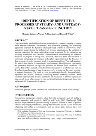
  • 5. IDENTIFICATION OF REPETITIVE PROCESSES AT STEADY- AND UNSTEADY-STATE: TRANSFER FUNCTION POSTERS 797 projects, i.e., the drilling occurs on every well construction project. Such degree of repetitiveness eases comparison and data validation because a repetitive process tends to present patterns in smaller data portions. The case documentation provides details about inputs, outputs and brief explanations of the process parameters. Nonetheless, the documentation does not include any mathematical representation of the processes other than the drilling parameters and other activities performed while drilling, which constitute subsystems. For instance, the work instructions to drill a segment of 28 meters on seabed:  Drill ahead 8 1/2" hole from 3684 m to 3712 m with 480 gpm, 1850 psi, 15- 25k WOB, 120 rpm, 15-20 kft.lbs torq. Perform surveys and downlinks as per directional driller instructions. Pump 15 bbl fine pill and 50 bbl hi-vis pill every two stand as per mud engineer instructions. The primary input, ‘drill ahead from 3684 m to 3712 m’, and the parameters, such as torque and rpm, directly affect the drilling process. However, the system view unifies the different parts of the system, i.e., the subsystems, into an effectual unit using a holistic perspective. The holistic perspective allows the creation of a system driven by a primary input while all others variables interact as subsystems of the main system. To fully establish a system, an input has to be applied to the process in order produce an output. Accordingly, the input, u(t), consists of a drilling ahead depth goal, e.g., 3712 meters, that is applied to the drilling process, producing the output, y(t), that is the actual depth, in meters. In the process, G(t), the drilling crew responds to the drilling ahead goal by drilling and performing related tasks, which increases the actual well depth over time until reaching the drilling depth goal. Then, a new drill ahead goal is set, and the process performs the cycle. The sample data corresponds with a well depth increase from 3305 to 3700 meters at a variable rate based on operational choices. The 181 samples represent the hourly input and process behavior response, i.e., output. The input and output data are cumulative due to physical restrictions. In other words, it is impossible to drill from 3435 meters without prior drilling from the seabed at 924 meters from water level to 3435 meters in the hole. Consequently the drill ahead goal as well as the actual depth values are always greater than the previous values. Figure 1 displays the general system representation of the process with its measured input and output, drill ahead goal and actual depth respectively. Two criteria guided the choice of drilling goal as input. The first criterion is that the drill ahead goal is the primarily directive to achieve the objective of the project, setting the peace to build the well. The drill ahead goal is an adaptive plan in which the team has to examine the current conditions of the well and determine the best drill ahead goal. It relies on guidelines and procedures but in the end its a human decision. The second criterionis that this particular arrangement illustrates the number of items arriving in a queuing system at time t. Additionally, the output represents the number of items departing in the queuing system at time t. Such input-output arrangement is instrumental to adapt manufacturing-based models such as the Little’s Law (Little, 1961) to construction in further research.
  • 6. Ricardo Antunes, Vicente A. González, and Kenneth Walsh 798 Proceedings IGLC-23, July 2015 |Perth, Australia Figure 1. System representation of the case study INITIAL MODELING APPROACH A simple model is attempted initially before progressing to more complex structures until reaching the required model accuracy. Simpler models are easier to interpret, a desired feature in this study. However, if that model unsatisfactorily simulates the measured data, it may be necessary to use more complex models. The simpler system identification approach is the transfer function. Hence, transfer function might be a good starting point in order to identify, model and understand the behavior of a system. The sample data was partitioned in nine combinations representing nine stages in time, as shown in Figure 1. The first partition is at the 20th hour. Therefore, the data from zero to 20 hours was used as estimation data for G1, and from 21 to 181 hours as the validation data. The second partition happens at 40 hours mark. In the same way, the estimation for G2 is composed of the data from zero to 40 hours mark, and the validation is from the 41st to the 181st hour. This pattern repeats until the 180-time stamp. At this partition, almost the whole sample constitutes the estimation data, and only one sample is left for validation of G9. The model from this partition, G9, merely fits the estimation data once there is virtually no data that could be used to validate the model. Based on black-box trial-and-error approach, the model parameters of the transfer function of first-order (Ogata, 2010) were generated for each partition using the iterative prediction-error minimization algorithm (Ljung, 2010) from MATLAB’s System Identification Toolbox. A first-order transfer function eases the model interpretability. MODEL DEVELOPMENT Three transfer functions, which showed the lowest unfitness values, calculated by 100% – normalized root mean square (NRMSE) (Armstrong and Collopy, 1992; Ljung, 2010), were selected for each of the nine data partitions, constituting the best models. A perfect fit corresponds to zero meaning that the simulated or predicted model output is exactly the same as the measured data. MODEL QUALITY ASSESSMENT The initial models were later refined using the prediction-error minimization algorithm (Ljung, 1998). After refinement, the models that achieved the lowest unfitness values to each estimation data partition that they derived from were then validated using the remaining data of their partition. Figure 2 shows the quality measurements of the best models for each partition. The quality measurements are the percentage of validation and estimation data unfitness, Akaike's Final Prediction Error (FPE) (Jones, 1975), loss function (Berger, 1985) and mean squared normalized error performance function (MSE) (Poli and Cirillo, 1993). The quality measurements
  • 7. IDENTIFICATION OF REPETITIVE PROCESSES AT STEADY- AND UNSTEADY-STATE: TRANSFER FUNCTION POSTERS 799 are represented in the graph by ‘Val unfit’, ‘Est unfit’, FPE, ‘Loss Fcn’, and MSE respectively. Although, the model choice in this study is not mathematically based on FPE, loss function and MSE their values were calculated and shown providing an extra measurement of model quality. A variety of measurements is useful for comparing different models as well as comparing the models with different modeling approaches. Differently from the models one to seven, the models for the segments eight and nine present high unfit levels to their validation segments, 72,64% and impossible to calculate, respectively. For G8, the input-output relation of the validation data, shown in the segment eight to nine in Figure 2, is extremely distinct from the data used in the estimation, segment one to eight. For G9, there is only one sample remaining to validate the model. Hence, the model G9(s) = 0.6646 / (s + 0.6687) corresponds to the structure that better reproduces the sample data with about 93% fitness. Accordingly, G9 is used later to demonstrated the step response. Figure 2. Quality comparison of the models Despite the model G9 has the lowest unfitted data, ‘Est unfit’, almost the whole sample data was used to estimateG9. Hence, G9 already ‘knows’the data sample and for this reason cannot be used as a predictor. In order to illustrate the prediction accuracy of the models, the model with the largest ‘unknown’ data, i.e., G1 is used. Figure 3 shows the comparison of the measured data and model G1(t), result of inverse Laplace Transform ofG1(s) = 0.4193 / (s + 0.4103);the solid line is the measured output and the dashed line the model response with 9.5% unfitness. The transfer function G1(t), can represent the process input-output relationship with sufficient precision. Furthermore, the model is estimated at an early stage, around the initial 10% duration, independently of any previous process knowledge. Figure 3. Comparison between the G1 response and measured data STEP RESPONSE Figure 4(a) shows the step response for the model G9. The model reaches steady-state about the sixth hour for a threshold of absolute two percent about the final value. The step amplitude used as input, 2.06, is the average drilling goal ahead. The system responds to this input reaching and staying steady at the output peak, yp = 2.05, about 0 20 40 60 80 100 120 140 160 180 3300 3350 3400 3450 3500 3550 3600 3650 3700 y (t) = 0.4193e −0.4103 t * u(t) Time (hours) Actualdepth(meters) Estimation Prediction Actual output Model response
  • 8. Ricardo Antunes, Vicente A. González, and Kenneth Walsh 800 Proceedings IGLC-23, July 2015 |Perth, Australia the 16th hour, tp. In this case, the steady-state value is the peak value because it is the value that the system tends to when t→∞ (Mandal, 2006). The average drilling rate from the measured output data is 2.1 meters per hour approximately the model output at steady-state, with a three percent error. Consequently, the model represents the system at steady-state. Although, the transient response stands for a significant part of the system dynamics. The system has a transient response every time it starts or stops. Although it stays at the transient state when it need small corrections, as, for instance, to fit a casing pipe to secure the well. In this case, the system also has inputs as small as one. For this input, the average response of the system is 0.55 meters per hour. In order to assess the system transient response, a unitary step unit was introduced to the system producing the system response, as shown in Figure 4(b). The average response for the unitary input is achieved around one hour by the system indicating that the system is performing in the transient state. Figure 4. (a) 2.06 step response (b) Unit step response CONCLUSIONS The results of the model’s accuracy were explicit. The models were consistent with the modeling approach and methodology. The valid transfer functions obtained reliablydescribed the process behavior and presented evidence of their accuracy using a range of model quality measurements. These findings thus lend support to the use of transfer function as a valid model approach and analytical technique in order to describe the dynamic conditions of production in repetitive processes in projects. Accounting for transient responses, transfer function fulfills a gap left by network scheduling and queueing theory as well as linear and dynamic programming, which ignore the transient stage and assume that the process is at steady-state. Moreover, a transfer functions may act as a multi-level management tool. Because transfer functions provide an output function from an input function, they enable the creation of accurate plans rather than single actions and a throughput function, instead of a system position. Transfer functions may be used by site managers as a process descriptor to monitor and control low-level activities, as shown in Figure 3. Dynamic and accurate plans that respond to actual inputs can regain the trust of those conducting the project work on planning and scheduling. Moreover, the model simulation may be used in a means-ends analysis determining the best solution to a construction process, which frequently requires the optimization of resources to the detriment of shorter duration. In other words, managers may use the model adjusting the drill ahead goal plan until attaining the defined goal, supporting managers’
  • 9. IDENTIFICATION OF REPETITIVE PROCESSES AT STEADY- AND UNSTEADY-STATE: TRANSFER FUNCTION POSTERS 801 decision-making process. Once the managers are satisfied with both the drill ahead goal plan and the system’s outcome, the plan is executed. A transfer function may also be applied to represent higher levels, providing project managers a holistic view. Reliance on this method must be tempered, however because the case does not represent the general conditions of repetitive process in construction. There is a variety of construction processes that happen in different states, production runs, and different learning curves creating unique process’ characteristics. For instance, this study presents the analysis of system’s transient and steady-state response, but not unsteady-state because the case scenario does not have this characteristic. Although the model can be reused in similar processes as an initial model, a limitation places on the existence of the process’ input-output data. It means that the model accuracy cannot be evaluated until some data has been produced. Finally, the study explores several concepts that are unfamiliar to general construction managers at this point restricting its audience. Nevertheless, the search for and the aggregation of knowledge and expertise from different disciplines and technical fields constitutes the foremost forces driving the evolution in managerial sciences. FUTURE OUTCOMES Different system identification approaches can write equations for practically any process. However, only after extensive research about the dynamic conditions of production in project-driven systems the lack of knowledge about the transient and unsteady-state responses can be replaced by explanatory and mathematical laws to production in projects. In a further horizon, processes transient and unsteady-state will be understood and managed to generate an optimum process outcome. Being it reducing the transient time, and faster-moving processes to steady-state or applying unsteady-state processing techniques producing an average output above steady-state levels and then creating high-performance processes. REFERENCES Abdelhamid, T. S. 2004. The self-destruction and renewal of lean construction theory: A prediction from Boyd-s theory. In: Proc. 12th Ann. Conf. of the Int’l. Group for Lean Construction. Helsingør, Denmark, Aug. 3-5. Altmann, W. and Macdonald, D., 2005. Practical Process Control for Engineers and Technicians. Burlington, MA: Elsevier. Antunes, R. and Gonzalez, V., 2015. A production model for construction: A theoretical framework. Buildings, 5(1), pp. 209-228. Arditi, D., Tokdemir, O. B. and Suh, K., 2001. Effect of learning on line-of-balance scheduling. International Journal of Project Management, 19(5), pp. 265-277. Armstrong, J. S. and Collopy, F., 1992. Error measures for generalizing about forecasting methods: Empirical comparisons. International Journal of Forecasting, 8(1), pp. 69-80. Bapat, R. B., 2011. Linear Algebra and Linear Models. 3rd ed. New Delhi: Springer. Berger, J. O., 1985. Statistical Decision Theory and Bayesian Analysis. Springer Series in Statistics. New York: Springer. Bernold, L. E., 1989. Simulation of Nonsteady Construction Processes. Journal of Construction Engineering and Management, 115(2), pp. 163-178.
  • 10. Ricardo Antunes, Vicente A. González, and Kenneth Walsh 802 Proceedings IGLC-23, July 2015 |Perth, Australia Bertelsen, S. 2003a. Complexity- Construction in a New Perspective. In: Proc. 11th Ann. Conf. of the Int’l. Group for Lean Construction. Blacksburg, VA, Jul. 21- 24. Bertelsen, S. 2003b. Construction as a Complex System. In: Proc. 11th Ann. Conf. of the Int’l. Group for Lean Construction. Blacksburg, VA, Jul. 21-24 Billings, S. A., 2013. Nonlinear System Identification Narmax Methods in the Time, Frequency, and Spatio-Temporal Domains. West Sussex: John Wiley & Sons. Garnier, H. and Wang L. Eds. 2008. Identification of Continuous-time Models from Sampled Data. London: Springer-Verlag. González, V., Alarcón, L. F. and Molenaar, K., 2009. Multiobjective Design of Work-In-Process Buffer for Scheduling Repetitive Building Projects. Automation in Construction, 18(2), pp. 95-108. Hopp, W. J. and Spearman, M. L., 1996. Factory Physics: Foundations of Manufacturing Management. 2nd ed. New York: Irwin McGraw-Hill. Jones, R. H., 1975. Fitting Auto regressions. Journal of the American Statistical Association, 70(351), pp. 590-592. Laufer, A., 1997. Simultaneous management: Managing projects in a dynamic environment. New York: American Management Association. Little, J. D. C., 1961. A Proof for the Queuing Formula: L= λ W. Operations Research, 9(3), pp. 383-387. Ljung, L., 1998. System Identification: Theory for the User. Upper Saddle River, NJ: Pearson Education. Ljung, L., 2010. System Identification Toolbox 7. Reference. Natick, MA: Mathworks. Lumsden, P. 1968. The Line-of-balance method. Oxford: Pergamon Press, Industrial Training Division. Lutz, J. D. and Hijazi, A., 1993. Planning repetitive construction: Current practice. Construction Management and Economics, 11(2), pp.99-110. Mandal, A. K. 2006. Introduction to Control Engineering: Modeling, Analysis and Design. New Delhi: New Age International Publishers. McCray, G. E. and Purvis, R. L., 2002. Project management under uncertainty: the impact of heuristics and biases. Project Management Journal, 33(1), pp. 49-57. Mills, A., 2001. A systematic approach to risk management for construction. Structural Survey, 19(5), pp. 245-252. Ogata, K., 2010. Modern Control Engineering. 5th ed. Upper Saddle River, NJ: Prentice Hall. Poli, A. A. and Cirillo, M. C., 1993. On the use of the normalized mean square error in evaluating dispersion model performance. Atmospheric Environment. Part A. General Topics, 27(15), 2427-2434. Poshdar, M., González, V. A., Raftery, G. and Orozco, F., 2014. Characterization of Process Variability in Construction. Journal of Construction Engineering and Management, 140, (11) 05014009. Walsh, K. D., Sawhney, A. and Bashford, H. H., 2007. Production Equations for Unsteady-State Construction Processes. Journal of Construction Engineering and Management, 133(3), pp. 245-261.