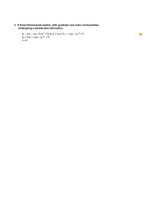
Mais conteúdo relacionado 1. A three-dimensional system, with quadratic and cubic nonlinearities,
undergoing a double-zero bifurcation.
q1 q1 q1 b1 q1 2 b2 q1 q1 b3 q1 2 q1 c1 q2 q1 3 0
..
q2 kq2 c2 q2 q1 3 0
k0
2. 2 my project.nb
Time scales and definitions
and definitions scales Time
OffGeneral::spell1
Notation`
Time scales
scales Time
SymbolizeT0 ; SymbolizeT1 ; SymbolizeT2 ; SymbolizeT3 ; SymbolizeT4 ;
timeScales T0 , T1 , T2 , T3 , T4 ;
dt1expr_ : Sum 2 Dexpr, timeScalesi 1, i, 0, maxOrder;
i
dt2expr_ : dt1dt1expr Expand . i_;imaxOrder 0;
conjugateRule A A, A A, , , Complex0, n_ Complex0, n;
displayRule q_i_,j_ a__ __ RowTimes MapIndexedD1
211 &, a, qi,j ,
A_i_ a__ __ RowTimes MapIndexedD1
21 &, a, Ai , q_i_,j_ __ qi,j , A_i_ __ Ai ;
3. my project.nb 3
Equations of motions
Equations motions of
Equations of motion
Equations motion of
EOM Subscriptq, 1 ''t
Subscriptq, 1 't Subscriptq, 1t b1 Subscriptq, 1t2
b2 Subscriptq, 1t Subscriptq, 1 't b3 Subscriptq, 1t2 Subscriptq, 1 't
c1 Subscriptq, 2t Subscriptq, 1t3 0,
Subscriptq, 2 't k Subscriptq, 2t
c2 Subscriptq, 2t Subscriptq, 1t3 0;
EOM TableForm
q1 t b1 q1 t2 c1 q1 t q2 t3 q1 t b2 q1 t q1 t b3 q1 t2 q1 t q1 t
k q2 t c2 q1 t q2 t3 q2 t 0
Ordering of the dampings
dampings of Ordering the
smorzrule , ;
Definition of the expansion of qi
Definition expansion of2 the qi
solRule qi_ Sum qi,j1 1, 2, 3, 4, 5, j, 0, 5 &;
j
2
multiScales
qi_ t qi timeScales, Derivativen_q_t dtnq timeScales, t T0 ;
Max order of the procedure
Max of order procedure the
maxOrder 4;
4. 4 my project.nb
Expansion and scaling of the equation
and equation Expansion of scaling the
q1 T0 , T1 , T2 , T3 , T4 , T5 . solRule
q1,1 T0 , T1 , T2 , T3 , T4 q1,2 T0 , T1 , T2 , T3 , T4 q1,3 T0 , T1 , T2 , T3 , T4
32 q1,4 T0 , T1 , T2 , T3 , T4 2 q1,5 T0 , T1 , T2 , T3 , T4 52 q1,6 T0 , T1 , T2 , T3 , T4
q1 't . multiScales
2 q1 0,0,0,0,1 T0 , T1 , T2 , T3 , T4
32 q1 0,0,0,1,0 T0 , T1 , T2 , T3 , T4 q1 0,0,1,0,0 T0 , T1 , T2 , T3 , T4
q1 0,1,0,0,0 T0 , T1 , T2 , T3 , T4 q1 1,0,0,0,0 T0 , T1 , T2 , T3 , T4
Scaling of the variables
of Scaling the variables
scaling Subscriptq, 1t Subscriptq, 1t,
Subscriptq, 2t Subscriptq, 2t, Subscriptq, 1 't Subscriptq, 1 't,
Subscriptq, 2 't Subscriptq, 2 't, Subscriptq, 1 ''t
Subscriptq, 1 ''t, Subscriptq, 2 ''t Subscriptq, 2 ''t
q1 t q1 t, q2 t q2 t, q1 t q1 t,
q2 t q2 t, q1 t q1 t, q2 t q2 t
Modification of the equations of motion : substitution of the rules.Representation.
EOMa EOM . scaling . multiScales . smorzrule . solRule TrigToExp ExpandAll .
n_;n3 0; EOMa . displayRule
2 D0 q1,1 52 D0 q1,2 3 D0 q1,3 D2 q1,1 32 D2 q1,2 2 D2 q1,3 52 D2 q1,4 3 D2 q1,5
0 0 0 0 0
52 D1 q1,1 3 D1 q1,2 2 32 D0 D1 q1,1 2 2 D0 D1 q1,2 2 52 D0 D1 q1,3 2 3 D0 D1 q1,4
2 D2 q1,1 52 D2 q1,2 3 D2 q1,3 3 D2 q1,1 2 2 D0 D2 q1,1 2 52 D0 D2 q1,2 2 3 D0 D2 q1,3
1 1 1
2 52 D1 D2 q1,1 2 3 D1 D2 q1,2 3 D2 q1,1 2 52 D0 D3 q1,1 2 3 D0 D3 q1,2 2 3 D1 D3 q1,1
2
2 3 D0 D4 q1,1 2 q1,1 2 D0 q1,1 b2 q1,1 52 D0 q1,2 b2 q1,1 3 D0 q1,3 b2 q1,1 52 D1 q1,1 b2 q1,1
3 D1 q1,2 b2 q1,1 3 D2 q1,1 b2 q1,1 2 b1 q2 3 D0 q1,1 b3 q2 3 c1 q3 52 q1,2
1,1 1,1 1,1
52 D0 q1,1 b2 q1,2 3 D0 q1,2 b2 q1,2 3 D1 q1,1 b2 q1,2 2 52 b1 q1,1 q1,2 3 b1 q2
1,2
3 q1,3 3 D0 q1,1 b2 q1,3 2 3 b1 q1,1 q1,3 3 3 c1 q2 q2,1 3 3 c1 q1,1 q2 3 c1 q3 0,
1,1 2,1 2,1
D0 q2,1 32 D0 q2,2 2 D0 q2,3 52 D0 q2,4 3 D0 q2,5 32 D1 q2,1 2 D1 q2,2 52 D1 q2,3
3 D1 q2,4 2 D2 q2,1 52 D2 q2,2 3 D2 q2,3 52 D3 q2,1 3 D3 q2,2 3 D4 q2,1 3 c2 q3 k q2,1
1,1
3 3 c2 q2 q2,1 3 3 c2 q1,1 q2 3 c2 q3 k 32 q2,2 k 2 q2,3 k 52 q2,4 k 3 q2,5 0
1,1 2,1 2,1
5. my project.nb 5
EOMb ExpandEOMa1, 1 0, ExpandEOMa2, 1 0; EOMb . displayRule
32 D0 q1,1 2 D0 q1,2 52 D0 q1,3 D2 q1,1 D2 q1,2 32 D2 q1,3 2 D2 q1,4 52 D2 q1,5
0 0 0 0 0
2 D1 q1,1 52 D1 q1,2 2 D0 D1 q1,1 2 32 D0 D1 q1,2 2 2 D0 D1 q1,3 2 52 D0 D1 q1,4
32 D2 q1,1 2 D2 q1,2 52 D2 q1,3 52 D2 q1,1 2 32 D0 D2 q1,1 2 2 D0 D2 q1,2 2 52 D0 D2 q1,3
1 1 1
2 2 D1 D2 q1,1 2 52 D1 D2 q1,2 52 D2 q1,1 2 2 D0 D3 q1,1 2 52 D0 D3 q1,2 2 52 D1 D3 q1,1
2
2 52 D0 D4 q1,1 32 q1,1 32 D0 q1,1 b2 q1,1 2 D0 q1,2 b2 q1,1 52 D0 q1,3 b2 q1,1 2 D1 q1,1 b2 q1,1
52 D1 q1,2 b2 q1,1 52 D2 q1,1 b2 q1,1 32 b1 q2 52 D0 q1,1 b3 q2 52 c1 q3 2 q1,2
1,1 1,1 1,1
2 D0 q1,1 b2 q1,2 52 D0 q1,2 b2 q1,2 52 D1 q1,1 b2 q1,2 2 2 b1 q1,1 q1,2 52 b1 q2 52 q1,3
1,2
52 D0 q1,1 b2 q1,3 2 52 b1 q1,1 q1,3 3 52 c1 q2 q2,1 3 52 c1 q1,1 q2 52 c1 q3 0,
1,1 2,1 2,1
D0 q2,1 D0 q2,2 32 D0 q2,3 2 D0 q2,4 52 D0 q2,5 D1 q2,1 32 D1 q2,2 2 D1 q2,3 52 D1 q2,4
32 D2 q2,1 2 D2 q2,2 52 D2 q2,3 2 D3 q2,1 52 D3 q2,2 52 D4 q2,1 52 c2 q3 k
1,1 q2,1
3 52
c2 q2
1,1 q2,1 3 52
c2 q1,1 q2
2,1 52
c2 q3
2,1 k q2,2 k 32
q2,3 k q2,4 k
2 52
q2,5 0
Separation of the coefficients of the powers of
coefficients of3 powers Separation the2
eqEps RestThreadCoefficientListSubtract , 2 0 & EOMb Transpose;
1
Definition of the equations at orders of and representation
and at Definition equations of2 orders representation the
eqOrderi_ : 1 & eqEps1 . q_k_,1 qk,i
1 & eqEps1 . q_k_,1 qk,i 1 & eqEpsi Thread
6. 6 my project.nb
Pertubation equations
equations Pertubation
.
.
eqOrder1 displayRule
.
eqOrder2 displayRule
.
eqOrder3 displayRule
.
eqOrder4 displayRule
eqOrder5 displayRule
D2 q1,1 0, D0 q2,1 k q2,1 0
0
D2 q1,2 2 D0 D1 q1,1 , D0 q2,2 k q2,2 D1 q2,1
0
D2 q1,3 D0 q1,1 2 D0 D1 q1,2 D2 q1,1 2 D0 D2 q1,1 q1,1 D0 q1,1 b2 q1,1 b1 q2 ,
D0 q2,3 k q2,3 D1 q2,2 D2 q2,1
0 1 1,1
D2 q1,4 D0 q1,2 D1 q1,1 2 D0 D1 q1,3 D2 q1,2 2 D0 D2 q1,2 2 D1 D2 q1,1 2 D0 D3 q1,1 D0 q1,2 b2 q1,1
D1 q1,1 b2 q1,1 q1,2 D0 q1,1 b2 q1,2 2 b1 q1,1 q1,2 , D0 q2,4 k q2,4 D1 q2,3 D2 q2,2 D3 q2,1
0 1
D2 q1,5 D0 q1,3 D1 q1,2 2 D0 D1 q1,4 D2 q1,3 D2 q1,1
0 1
2 D0 D2 q1,3 2 D1 D2 q1,2 D2 q1,1 2 D0 D3 q1,2 2 D1 D3 q1,1 2 D0 D4 q1,1 D0 q1,3 b2 q1,1
2
D1 q1,2 b2 q1,1 D2 q1,1 b2 q1,1 D0 q1,1 b3 q1,1 c1 q1,1 D0 q1,2 b2 q1,2 D1 q1,1 b2 q1,2
2 3
b1 q1,2 q1,3 D0 q1,1 b2 q1,3 2 b1 q1,1 q1,3 3 c1 q1,1 q2,1 3 c1 q1,1 q2,1 c1 q2,1 ,
2 2 2 3
D0 q2,5 k q2,5 D1 q2,4 D2 q2,3 D3 q2,2 D4 q2,1 c2 q1,1 3 c2 q1,1 q2,1 3 c2 q1,1 q2,1 c2 q2,1
3 2 2 3
7. my project.nb 7
First Order Problem
First Order Problem
linearSys 1 & eqOrder1;
linearSys . displayRule TableForm
D2 q1,1
0
D0 q2,1 k q2,1
Formal solution of the First Order Problem generating solution
generating Order Problem solution First Formal of solution the
sol1 q1,1 FunctionT0 , T1 , T2 , T3 , T4 , A1 T1 , T2 , T3 , T4 ,
q2,1 FunctionT0 , T1 , T2 , T3 , T4 , 0
q1,1 FunctionT0 , T1 , T2 , T3 , T4 , A1 T1 , T2 , T3 , T4 , q2,1 FunctionT0 , T1 , T2 , T3 , T4 , 0
8. 8 my project.nb
Second Order Problem
Order Problem Second
Substitution of the solution on the Second Order Problem and representation
and Order Problem representation of on Second solution Substitution the2
eqOrder2 . displayRule
D2 q1,2 2 D0 D1 q1,1 , D0 q2,2 k q2,2 D1 q2,1
0
order2Eq eqOrder2 . sol1 ExpandAll;
order2Eq . displayRule
D2 q1,2 0, D0 q2,2 k q2,2 0
0
we eliminate secular terms then we obtain
eliminate obtain secular terms then we2
sol2 q1,2 FunctionT0 , T1 , T2 , T3 , T4 , 0 , q2,2 FunctionT0 , T1 , T2 , T3 , T4 , 0
q1,2 FunctionT0 , T1 , T2 , T3 , T4 , 0, q2,2 FunctionT0 , T1 , T2 , T3 , T4 , 0
9. my project.nb 9
Third Order Problem
Order Problem Third
Substitution in the Third Order Equations
Equations Order in Substitution the Third
order3Eq eqOrder3 . sol1 . sol2 ExpandAll;
order3Eq . displayRule
D2 q1,3 D2 A1 A1 A2 b1 , D0 q2,3 k q2,3 0
0 1 1
ST31 order3Eq, 2 & 1;
ST31 . displayRule
D2 A1 A1 A2 b1
1 1
SCond3 ST31 0;
SCond3 . displayRule
D2 A1 A1 A2 b1 0
1 1
SCond3
A1 T1 , T2 , T3 , T4 b1 A1 T1 , T2 , T3 , T4 2 A1 2,0,0,0 T1 , T2 , T3 , T4 0
A1 T1 , T2 , T3 , T4 b1 A1 T1 , T2 , T3 , T4 2 A1 2,0,0,0 T1 , T2 , T3 , T4 0
A1 T1 , T2 , T3 , T4 b1 A1 T1 , T2 , T3 , T4 2 A1 2,0,0,0 T1 , T2 , T3 , T4 0
A1 T1 , T2 , T3 , T4 b1 A1 T1 , T2 , T3 , T4 2 A1 2,0,0,0 T1 , T2 , T3 , T4 0
A1 T1 , T2 , T3 , T4 b1 A1 T1 , T2 , T3 , T4 2 A1 2,0,0,0 T1 , T2 , T3 , T4 0
SCond3Rule1
SolveSCond3, A1 2,0,0,0 T1 , T2 , T3 , T4 1 ExpandAll Simplify Expand;
SCond3Rule1 . displayRule
D2 A1 A1 A2 b1
1 1
sol3 q1,3 FunctionT0 , T1 , T2 , T3 , T4 , 0 , q2,3 FunctionT0 , T1 , T2 , T3 , T4 , 0
q1,3 FunctionT0 , T1 , T2 , T3 , T4 , 0, q2,3 FunctionT0 , T1 , T2 , T3 , T4 , 0
10. 10 my project.nb
Fourth Order Problem
Fourth Order Problem
Substitution in the Fourth Order Equations
Equations Order Fourth in Substitution the
order4Eq eqOrder4 . sol1 . sol2 . sol3 ExpandAll;
order4Eq . displayRule
D2 q1,4 D1 A1 2 D1 D2 A1 D1 A1 A1 b2 , D0 q2,4 k q2,4 0
0
ST41 order4Eq, 2 & 1;
ST41 . displayRule
D1 A1 2 D1 D2 A1 D1 A1 A1 b2
SCond4 ST41 0;
SCond4 . displayRule
D1 A1 2 D1 D2 A1 D1 A1 A1 b2 0
SCond4
A1 1,0,0,0 T1 , T2 , T3 , T4
b2 A1 T1 , T2 , T3 , T4 A1 1,0,0,0 T1 , T2 , T3 , T4 2 A1 1,1,0,0 T1 , T2 , T3 , T4 0
A1 1,0,0,0 T1 , T2 , T3 , T4
b2 A1 T1 , T2 , T3 , T4 A1 1,0,0,0 T1 , T2 , T3 , T4 2 A1 1,1,0,0 T1 , T2 , T3 , T4 0
A1 1,0,0,0 T1 , T2 , T3 , T4
b2 A1 T1 , T2 , T3 , T4 A1 1,0,0,0 T1 , T2 , T3 , T4 2 A1 1,1,0,0 T1 , T2 , T3 , T4 0
A1 1,0,0,0 T1 , T2 , T3 , T4
b2 A1 T1 , T2 , T3 , T4 A1 1,0,0,0 T1 , T2 , T3 , T4 2 A1 1,1,0,0 T1 , T2 , T3 , T4 0
A1 1,0,0,0 T1 , T2 , T3 , T4
b2 A1 T1 , T2 , T3 , T4 A1 1,0,0,0 T1 , T2 , T3 , T4 2 A1 1,1,0,0 T1 , T2 , T3 , T4 0
SCond4Rule1
SolveSCond4, A1 1,1,0,0 T1 , T2 , T3 , T4 1 ExpandAll Simplify Expand;
SCond4Rule1 . displayRule
D1 D2 A1 D1 A1 A1 b2
D1 A1 1
2 2
SCond3Rule1 . displayRule
D2 A1 A1 A2 b1
1 1
SCond3Rule1
A1 2,0,0,0 T1 , T2 , T3 , T4 A1 T1 , T2 , T3 , T4 b1 A1 T1 , T2 , T3 , T4 2
A1 2,0,0,0 T1 , T2 , T3 , T4 A1 T1 , T2 , T3 , T4 b1 A1 T1 , T2 , T3 , T4 2
A1 2,0,0,0 T1 , T2 , T3 , T4 A1 T1 , T2 , T3 , T4 b1 A1 T1 , T2 , T3 , T4 2
11. my project.nb 11
SCond4Rule1
A1 1,1,0,0 T1 , T2 , T3 , T4
A1 1,0,0,0 T1 , T2 , T3 , T4 b2 A1 T1 , T2 , T3 , T4 A1 1,0,0,0 T1 , T2 , T3 , T4
1 1
2 2
A1 1,1,0,0 T1 , T2 , T3 , T4
A1 1,0,0,0 T1 , T2 , T3 , T4 b2 A1 T1 , T2 , T3 , T4 A1 1,0,0,0 T1 , T2 , T3 , T4
1 1
2 2
A1 1,1,0,0 T1 , T2 , T3 , T4
A1 1,0,0,0 T1 , T2 , T3 , T4 b2 A1 T1 , T2 , T3 , T4 A1 1,0,0,0 T1 , T2 , T3 , T4
1 1
2 2
A1 1,1,0,0 T1 , T2 , T3 , T4
A1 1,0,0,0 T1 , T2 , T3 , T4 b2 A1 T1 , T2 , T3 , T4 A1 1,0,0,0 T1 , T2 , T3 , T4
1 1
2 2
A1 1,1,0,0 T1 , T2 , T3 , T4
A1 1,0,0,0 T1 , T2 , T3 , T4 b2 A1 T1 , T2 , T3 , T4 A1 1,0,0,0 T1 , T2 , T3 , T4
1 1
2 2
2 A1 1,1,0,0 T1 , T2 , T3 , T4 A1 2,0,0,0 T1 , T2 , T3 , T4 . SCond3Rule1 . SCond4Rule1
A1 T1 , T2 , T3 , T4 b1 A1 T1 , T2 , T3 , T4 2
A1 1,0,0,0 T1 , T2 , T3 , T4 b2 A1 T1 , T2 , T3 , T4 A1 1,0,0,0 T1 , T2 , T3 , T4
1 1
2
2 2
TimeRule1 A1 T1 , T2 , T3 , T4 A1 t, A1 1,0,0,0 T1 , T2 , T3 , T4 A1 't
A1 T1 , T2 , T3 , T4 A1 t, A1 1,0,0,0 T1 , T2 , T3 , T4 A1 t
2 A1 1,1,0,0 T1 , T2 , T3 , T4 A1 2,0,0,0 T1 , T2 , T3 , T4 . SCond3Rule1 . SCond4Rule1 .
TimeRule1 A1 ''t
A1 t b1 A1 t2 2 A1 t b2 A1 t A1 t A1 t
1 1
2 2
sol4 q1,4 FunctionT0 , T1 , T2 , T3 , T4 , 0 , q2,4 FunctionT0 , T1 , T2 , T3 , T4 , 0
q1,4 FunctionT0 , T1 , T2 , T3 , T4 , 0, q2,4 FunctionT0 , T1 , T2 , T3 , T4 , 0
12. 12 my project.nb
Fifth Order Problem
Fifth Order Problem
order5Eq eqOrder5 . sol1 . sol2 . sol3 . sol4 ExpandAll;
order5Eq . displayRule
D2 q1,5 D2 A1 D2 A1 2 D1 D3 A1 D2 A1 A1 b2 A3 c1 , D0 q2,5 k q2,5 A3 c2
0 2 1 1
ST51 order5Eq, 2 & 1;
ST51 . displayRule
D2 A1 D2 A1 2 D1 D3 A1 D2 A1 A1 b2 A3 c1
2 1
SCond5 ST51 0;
SCond5 . displayRule
D2 A1 D2 A1 2 D1 D3 A1 D2 A1 A1 b2 A3 c1 0
2 1
SCond5
c1 A1 T1 , T2 , T3 , T4 3
A1 0,1,0,0 T1 , T2 , T3 , T4 b2 A1 T1 , T2 , T3 , T4 A1 0,1,0,0 T1 , T2 , T3 , T4
A1 0,2,0,0 T1 , T2 , T3 , T4 2 A1 1,0,1,0 T1 , T2 , T3 , T4 0
c1 A1 T1 , T2 , T3 , T4 3 A1 0,1,0,0 T1 , T2 , T3 , T4 b2 A1 T1 , T2 , T3 , T4
A1 0,1,0,0 T1 , T2 , T3 , T4 A1 0,2,0,0 T1 , T2 , T3 , T4 2 A1 1,0,1,0 T1 , T2 , T3 , T4 0
c1 A1 T1 , T2 , T3 , T4 3
A1 0,1,0,0 T1 , T2 , T3 , T4 b2 A1 T1 , T2 , T3 , T4 A1 0,1,0,0 T1 , T2 , T3 , T4
A1 0,2,0,0 T1 , T2 , T3 , T4 2 A1 1,0,1,0 T1 , T2 , T3 , T4 0
SCond5Rule1
SolveSCond5, A1 0,2,0,0 T1 , T2 , T3 , T4 1 ExpandAll Simplify Expand;
SCond5Rule1 . displayRule
D2 A1 D2 A1 2 D1 D3 A1 D2 A1 A1 b2 A3 c1
2 1
SCond5Rule1
A1 0,2,0,0 T1 , T2 , T3 , T4 c1 A1 T1 , T2 , T3 , T4 3 A1 0,1,0,0 T1 , T2 , T3 , T4
b2 A1 T1 , T2 , T3 , T4 A1 0,1,0,0 T1 , T2 , T3 , T4 2 A1 1,0,1,0 T1 , T2 , T3 , T4
A1 0,2,0,0 T1 , T2 , T3 , T4 c1 A1 T1 , T2 , T3 , T4 3 A1 0,1,0,0 T1 , T2 , T3 , T4
b2 A1 T1 , T2 , T3 , T4 A1 0,1,0,0 T1 , T2 , T3 , T4 2 A1 1,0,1,0 T1 , T2 , T3 , T4
A1 0,2,0,0 T1 , T2 , T3 , T4 c1 A1 T1 , T2 , T3 , T4 3 A1 0,1,0,0 T1 , T2 , T3 , T4
b2 A1 T1 , T2 , T3 , T4 A1 0,1,0,0 T1 , T2 , T3 , T4 2 A1 1,0,1,0 T1 , T2 , T3 , T4
c1 c2 A1 T1 , T2 , T3 , T4 3
A1 0,2,0,0 T1 , T2 , T3 , T4 A1 0,1,0,0 T1 , T2 , T3 , T4
k
b2 A1 T1 , T2 , T3 , T4 A1 0,1,0,0 T1 , T2 , T3 , T4 2 A1 1,0,1,0 T1 , T2 , T3 , T4
c1 c2 A1 T1 , T2 , T3 , T4 3
A1 0,2,0,0 T1 , T2 , T3 , T4 A1 0,1,0,0 T1 , T2 , T3 , T4
b2 A1 T1 , T2 , T3 , T4 A1 0,1,0,0 T1 , T2 , T3 , T4 2 A1 1,0,1,0 T1 , T2 , T3 , T4
k
13. my project.nb 13
A1 0,2,0,0 T1 , T2 , T3 , T4 2 A1 1,0,1,0 T1 , T2 , T3 , T4 . SCond5Rule1 . TimeRule1
c1 A1 t3 A1 0,1,0,0 T1 , T2 , T3 , T4 b2 A1 t A1 0,1,0,0 T1 , T2 , T3 , T4
sol5 q1,5 FunctionT0 , T1 , T2 , T3 , T4 , 0 , q2,5 FunctionT0 , T1 , T2 , T3 , T4 ,
A1 3 c2
k
q1,5 FunctionT0 , T1 , T2 , T3 , T4 , 0, q2,5 FunctionT0 , T1 , T2 , T3 , T4 ,
A3 c2
1
k
14. 14 my project.nb
Bifurcation equations and fixed points
and Bifurcation equations fixed points
TimeRule2 A1 0,1,0,0 T1 , T2 , T3 , T4 0
A1 0,1,0,0 T1 , T2 , T3 , T4 0
RBFCE A1 0,2,0,0 T1 , T2 , T3 , T4 2 A1 1,0,1,0 T1 , T2 , T3 , T4
2 A1 1,1,0,0 T1 , T2 , T3 , T4 A1 2,0,0,0 T1 , T2 , T3 , T4 . SCond3Rule1 .
SCond4Rule1 . SCond5Rule1 . TimeRule1 . TimeRule2 A1 ''t
A1 t b1 A1 t2 c1 A1 t3 2 A1 t b2 A1 t A1 t A1 t
1 1
2 2
15. my project.nb 15
Fixed points
Perfect system
Perfect system
perfectsyst A1 t 0, A1 t 0
A1 t 0, A1 t 0
fix1 RBFCE . perfectsyst
A1 t b1 A1 t2 c1 A1 t3
fixpoint1 fix1 0;
fixpoint1 . displayRule
A1 A2 b1 A3 c1 0
1 1
fixpoint1
A1 t b1 A1 t2 c1 A1 t3 0
scalingRule2 A1 2,0,0,0 T1 , T2 , T3 , T4 A1 t
A1 2,0,0,0 T1 , T2 , T3 , T4 A1 t
A1 2,0,0,0 T1 , T2 , T3 , T4 A1 t
Solvefixpoint1, A1 t
A1 2,0,0,0 T1 , T2 , T3 , T4 A1 t
A1 t 0, A1 t , A1 t
b1 b2 4 c1
1 b1 b2 4 c1
1
2 c1 2 c1
16. 16 my project.nb
Reconstitution of the equation of the motion
Stepx1 A1 T1 , T2 , T3 , T4
A1 T1 , T2 , T3 , T4
c2 A1 T1 , T2 , T3 , T4 3
Stepy1
k
c2 A1 T1 , T2 , T3 , T4 3
k
ScalingRule1 A1 T1 , T2 , T3 , T4 A1 t
A1 T1 , T2 , T3 , T4 A1 t
x t A1 T1 , T2 , T3 , T4 . ScalingRule1
A1 t
scalingRule2
D1 A1 1,0,0,0 T1 , T2 , T3 , T4 A1 t , D2 A1 T1 , T2 , T3 , T4 0 , D1 A1 T1 , T2 , T3 , T4 A1 t
D1 A1 1,0,0,0 T1 , T2 , T3 , T4 A1 t, D2 A1 T1 , T2 , T3 , T4 0, D1 A1 T1 , T2 , T3 , T4 A1 t
c2 A1 T1 , T2 , T3 , T4 3
y t . scalingRule2 . ScalingRule1
k
c2 A1 t3
k
17. my project.nb 17
Numerical integrations
Numerical values for the perfect system
for Numerical perfect system the values
c1 1, k 2, b3
1
, b1 1, b2 1, c2 1, 0.01, 0.9
2
1, 2,
1
, 1, 1, 1, 0.01, 0.9
2
Time of integration
integration of Time
ti 500;
Numerical Intergations of the reconstitute
solution and study of the motion around the equilibrium points
and around equilibrium Intergations motion Numerical of2 points reconstitute solution study the3
solramep1 NDSolveRBFCE 0, A1 0 0.01, A1 0 0.01 ,
A1 t, A1 t, A1 t, t, 0, ti
A1 t InterpolatingFunction0., 500., t,
A1 t InterpolatingFunction0., 500., t,
A1 t InterpolatingFunction0., 500., t
18. 18 my project.nb
GraphicsArrayPlotSubscriptA, 1t . solramep1, t, 0, ti,
PlotStyle Thick, PlotRange Automatic, All, Frame True,
FrameLabel "t", "SubscriptBox"q", "1"t",
A1 t . solramep1, t, 0, ti,
Plot
PlotStyle Thick, PlotRange Automatic, Automatic,
Frame True,
FrameLabel "t",
l TableSubscriptA, 1t . solramep1,
"SubscriptBoxOverscriptBox"q", ".", "1"t"
A1 t . solramep1, t, 0, ti;
ListPlotTableExtractlj, 1, 1, Extractlj, 2, 1, j,
1, ti 1, Joined True
0.15
0.2 0.10
0.05
q1 t
q1 t
0.0 0.00
0.05
0.2
0.10
0.4 0.15
0 100 200 300 400 500 0 100 200 300 400 500
t t
0.15
0.10
0.05
0.15 0.10 0.05 0.05 0.10 0.15
0.05
0.10
0.15
0.20
Graphics of the reconstituted solution
Graphics of reconstituted solution the
19. my project.nb 19
solramep1 NDSolveRBFCE 0, A1 0 0.01, A1 0 0.01 ,
A1 t, A1 t, A1 t, t, 0, ti
GraphicsArrayPlotA1 t . solramep1, t, 0, ti, PlotStyle Thick,
PlotRange Automatic, 3.8, 3.8, Frame True, FrameLabel "t", "xt",
c2 A1 t3
Plot . solramep1, t, 0, ti, PlotStyle Thick,
k
PlotRange Automatic, 2.6, 2.4, Frame True, FrameLabel "t", "yt"
A1 t InterpolatingFunction0., 500., t,
A1 t InterpolatingFunction0., 500., t,
A1 t InterpolatingFunction0., 500., t
3 2
2 1
1
xt
yt
0 0
1 1
2
3 2
0 100 200 300 400 500 0 100 200 300 400 500
t t
Numerical Intergations of the original equations
equations Intergations Numerical of original the
solorig1 NDSolveJoinEOM, q1 0 0.01, q2 0 0.01, q1 '0 0.01,
q1 t, q2 t, t, 0, ti, MaxSteps 1 000 000
q1 t InterpolatingFunction0., 500., t,
q2 t InterpolatingFunction0., 500., t
GraphicsArrayPlotq1 t . solorig1, t, 0, ti, PlotStyle Thick,
PlotRange Automatic, 0.8, 0.8, Frame True, FrameLabel "t", "q1 t",
Plotq2 t . solorig1, t, 0, ti, PlotStyle Thick,
PlotRange Automatic, 0.6, 0.4, Frame True, FrameLabel "t", "q2 t"
0.4
0.5
0.2
q1 t
0.0
q2 t
0.0
0.2
0.5 0.4
0.6
0 100 200 300 400 500 0 100 200 300 400 500
t t
20. 20 my project.nb
Another Example
Numerical values for the perfect syst em
c1 0.5, k 1, b3 , b1 0.5, b2 0.5, c2 0.5, 0.01, 0.9
1
2
Time of integration
ti 500;
Numerical Intergations of the reconstitute
solramep1 NDSolveRBFCE 0, A1 0 0.01, A1 0 0.01 ,
solution and study of the motion around the equilibrium points
A1 t, A1 t, A1 t, t, 0, ti
GraphicsArrayPlotSubscriptA, 1t . solramep1, t, 0, ti,
PlotStyle Thick, PlotRange Automatic, All, Frame True,
FrameLabel "t", "SubscriptBox"q", "1"t",
A1 t . solramep1, t, 0, ti,
Plot
PlotStyle Thick, PlotRange Automatic, Automatic,
Frame True,
FrameLabel "t",
l TableSubscriptA, 1t . solramep1,
"SubscriptBoxOverscriptBox"q", ".", "1"t"
A1 t . solramep1, t, 0, ti;
ListPlotTableExtractlj, 1, 1, Extractlj, 2, 1, j,
1, ti 1, Joined True
Another Example
em for Numerical perfect syst the values
0.5, 1,
1
, 0.5, 0.5, 0.5, 0.01, 0.9
2
integration of Time
and around equilibrium Intergations motion Numerical of2 points reconstitute solution study the3
A1 t InterpolatingFunction0., 500., t,
A1 t InterpolatingFunction0., 500., t,
A1 t InterpolatingFunction0., 500., t
0.2 0.15
0.1 0.10
0.05
q1 t
q1 t
0.0 0.00
0.05
0.1 0.10
0.15
0.2
0 100 200 300 400 500 0 100 200 300 400 500
t t
21. my project.nb 21
0.15
0.10
0.05
0.20 0.15 0.10 0.05 0.05 0.10 0.15
0.05
0.10
0.15
Graphics of the reconstituted solution
Graphics of reconstituted solution the
solramep1 NDSolveRBFCE 0, A1 0 0.01, A1 0 0.01 ,
A1 t, A1 t, A1 t, t, 0, ti
GraphicsArrayPlotA1 t . solramep1, t, 0, ti, PlotStyle Thick,
PlotRange Automatic, 3.8, 3.8, Frame True, FrameLabel "t", "xt",
c2 A1 t3
Plot . solramep1, t, 0, ti, PlotStyle Thick,
k
PlotRange Automatic, 2.6, 2.4, Frame True, FrameLabel "t", "yt"
A1 t InterpolatingFunction0., 500., t,
A1 t InterpolatingFunction0., 500., t,
A1 t InterpolatingFunction0., 500., t
3 2
2 1
1
xt
yt
0 0
1 1
2
3 2
0 100 200 300 400 500 0 100 200 300 400 500
t t
22. 22 my project.nb
solorig1 NDSolveJoinEOM, q1 0 0.01, q2 0 0.01, q1 '0 0.01,
Numerical Intergations of the original equations
q1 t, q2 t, t, 0, ti, MaxSteps 1 000 000
GraphicsArrayPlotq1 t . solorig1, t, 0, ti, PlotStyle Thick,
PlotRange Automatic, 0.8, 0.8, Frame True, FrameLabel "t", "q1 t",
Plotq2 t . solorig1, t, 0, ti, PlotStyle Thick,
PlotRange Automatic, 0.6, 0.4, Frame True, FrameLabel "t", "q2 t"
equations Intergations Numerical of original the
q1 t InterpolatingFunction0., 500., t,
q2 t InterpolatingFunction0., 500., t
0.4
0.5
0.2
q1 t
0.0
q2 t
0.0
0.2
0.5 0.4
0.6
0 100 200 300 400 500 0 100 200 300 400 500
t t