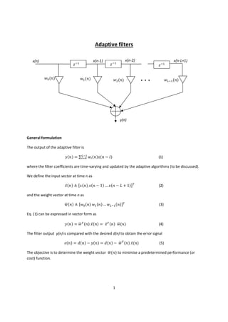
1. Adaptive filters
x(n)
‫ݓ‬଴ ሺ݊ሻ
‫ି ݖ‬ଵ
x(n-1)
‫ݓ‬ଵ ሺ݊ሻ
‫ି ݖ‬ଵ
‫ି ݖ‬ଵ
x(n-2)
‫ݓ‬ଶ ሺ݊ሻ
x(n-L+1)
‫ݓ‬௅ିଵ ሺ݊ሻ
...
y(n)
General formulation
The output of the adaptive filter is
‫ݕ‬ሺ݊ሻ = ∑௅ିଵ ‫ݓ‬௟ ሺ݊ሻ‫ݔ‬ሺ݊ − ݈ሻ
௟ୀ଴
(1)
where the filter coefficients are time-varying and updated by the adaptive algorithms (to be discussed).
We define the input vector at time n as
‫ ̅ݔ‬ሺ݊ሻ ≜ ሾ‫ݔ‬ሺ݊ሻ ‫ݔ‬ሺ݊ − 1ሻ … ‫ݔ‬ሺ݊ − ‫1 + ܮ‬ሻሿ்
(2)
‫ ݓ‬ሺ݊ሻ ≜ ሾ‫ݓ‬଴ ሺ݊ሻ ‫ݓ‬ଵ ሺ݊ሻ … ‫ݓ‬௅ିଵ ሺ݊ሻሿ்
ഥ
(3)
ഥሺ݊ሻ
‫ݕ‬ሺ݊ሻ = ‫ ் ݓ‬ሺ݊ሻ ‫ ̅ݔ‬ሺ݊ሻ = ‫ ் ̅ݔ‬ሺ݊ሻ ‫ݓ‬
ഥ
(4)
݁ሺ݊ሻ = ݀ሺ݊ሻ − ‫ݕ‬ሺ݊ሻ = ݀ሺ݊ሻ − ‫ ் ݓ‬ሺ݊ሻ ‫ ̅ݔ‬ሺ݊ሻ
ഥ
(5)
and the weight vector at time n as
Eq. (1) can be expressed in vector form as
The filter output y(n) is compared with the desired d(n) to obtain the error signal
The objective is to determine the weight vector ‫ݓ‬
ഥሺ݊ሻ to minimise a predetermined performance (or
cost) function.
1

2. Optimization
The most commonly used performance function is based on the mean squared error (MSE) defined as
ߦሺ݊ሻ ≜ ‫ܧ‬ሾ݁ ଶ ሺ݊ሻሿ
(6)
ത ഥሺ݊ሻ
ߦሺ݊ሻ = ‫ܧ‬ሾ݀ଶ ሺ݊ሻሿ − 2 ‫ ݓ ் ̅݌‬ሺ݊ሻ + ‫ ் ݓ‬ሺ݊ሻ ܴ ‫ݓ‬
ഥ
ഥ
(7)
The MSE function determined by substituting eq. (5) in eq. (6) can be expressed as
where ‫ ̅݌‬is the autocorrelation vector defined as
‫ܧ ≜ ̅݌‬ሾ݀ሺ݊ሻ‫ ̅ݔ‬ሺ݊ሻሿ = ሾ‫ݎ‬ௗ௫ ሺ0ሻ ‫ݎ‬ௗ௫ ሺ1ሻ … ‫ݎ‬ௗ௫ ሺ‫1 − ܮ‬ሻሿ்
and
‫ݎ‬ௗ௫ ሺ݇ሻ ≜ ‫ܧ‬ሾ݀ሺ݊ + ݇ሻ‫ݔ‬ሺ݊ሻሿ
is the autocorrelation function between ݀ሺ݊ሻ and ‫ݔ‬ሺ݊ሻ.
ത
ܴ is the input autocorrelation matrix defined as
‫ݎ‬௫௫ ሺ1ሻ
… ‫ݎ‬௫௫ ሺ‫1 − ܮ‬ሻ
‫ݎ‬௫௫ ሺ0ሻ
‫ݎ‬௫௫ ሺ1ሻ
‫ݎ‬௫௫ ሺ0ሻ
… ‫ݎ‬௫௫ ሺ‫2 − ܮ‬ሻ
ܴ ≜ ‫ܧ‬ሾ‫ ̅ݔ‬ሺ݊ሻ‫ ் ̅ݔ‬ሺ݊ሻሿ = ൦
൪
⋮
⋮
⋱
⋮
‫ݎ‬௫௫ ሺ‫1 − ܮ‬ሻ ‫ݎ‬௫௫ ሺ‫2 − ܮ‬ሻ ⋯
‫ݎ‬௫௫ ሺ0ሻ
where ‫ݎ‬௫௫ is the autocorrelation function of ‫ݔ‬ሺ݊ሻ.
Steepest descent
The MSE in eq. (7) is a quadratic function of the weights. We can use a steepest descent method in order
to reach the minimum by following the negative gradient direction, in which the performance surface
has the greatest rate of decrease.
where ߤ is a step size.
‫1 + ݓ‬ሻ = ‫ ݓ‬ሺ݊ሻ − ∇ߦሺ݊ሻ
ഥሺ݊
ഥ
ఓ
ଶ
2
(8)

3. The LMS algorithm
In many practical applications, the statistics of d(n) and x(n) are unknown. Therefore, the steepest
descent method cannot be used directly since it assumes exact knowledge of the gradient vector. The
LMS algorithm uses the instantaneous error ݁ ଶ ሺ݊ሻ to estimate the Mean Squared Error (MSE).
ߦሺ݊ሻ ≜ ݁ ଶ ሺ݊ሻ
Therefore, the gradient used by the LMS algorithm can be written as
∇ߦሺ݊ሻ = ∇݁ ଶ ሺ݊ሻ = 2 ∙ ∇݁ሺ݊ሻ ∙ ݁ሺ݊ሻ
(9)
Since ݁ሺ݊ሻ = ݀ሺ݊ሻ − ‫ ் ݓ‬ሺ݊ሻ‫ ̅ݔ‬ሺ݊ሻ
ഥ
∇eሺnሻ = ∇൫݀ሺ݊ሻ − ‫ ் ݓ‬ሺ݊ሻ‫ ̅ݔ‬ሺ݊ሻ൯ = −xሺnሻ
ഥ
ത
Therefore, the gradient estimate of eq. (9) becomes
∇ߦሺ݊ሻ = −2 ∙ ݁ሺ݊ሻ ∙ ‫ ̅ݔ‬ሺ݊ሻ
By substituting this gradient estimate into the steepest descent algorithm of eq. (8), we have
‫ ݓ‬ሺ݊ + 1ሻ = ‫ݓ‬
ഥ
ഥሺ݊ሻ + ߤ ∙ ‫ ̅ݔ‬ሺ݊ሻ ∙ ݁ሺ݊ሻ
This is the well-known LMS algorithm. It is simple and does not require squaring, averaging, and
differentiating. The LMS structure is graphically depicted in the figure below.
d(n)
x(n)
‫ݓ‬
ഥሺ݊ሻ
+
y(n)
-
+
e(n)
LMS
Steps for the application of the LMS algorithm:
1. Determine ‫ ߤ ,ܮ‬and ‫ݓ‬
ഥሺ0ሻ , where L is the length of the filter, ߤ is the LMS step size, and ‫ ݓ‬ሺ0ሻ is
ഥ
the initial filter vector.
2. Compute the output of the adaptive filter as: ‫ݕ‬ሺ݊ሻ = ∑௅ିଵ ‫ݓ‬௟ ሺ݊ሻ‫ݔ‬ሺ݊ − ݈ሻ
௟ୀ଴
3. Compute the error signal ݁ሺ݊ሻ = ݀ሺ݊ሻ − ‫ݕ‬ሺ݊ሻ
4. Update the adaptive filter vector using the LMS algorithm
‫ݓ‬௟ ሺ݊ + 1ሻ = ‫ݓ‬௟ ሺ݊ሻ + ߤ ∙ ‫ݔ‬ሺ݊ − ݈ሻ ∙ ݁ሺ݊ሻ
3