A STUDY ON THE IMPACT OF TRANSPORT AND POWER INFRASTRUCTURE DEVELOPMENT ON TH...
Judi
1. International Review of Business Research Papers
Vol.3 No.2 June 2007, Pp. 162 - 183
Forecasting the Non – Oil GDP in the United Arab Emirates
by Using ARIMA Models
Yasmin Judi*
United Arab Emirates economy keeps exceeding the most optimistic
expectations, and even in times of political or economic crises, it was
able to absorb all shocks and bounce back, and it's becoming one of the
star performers of the Middle East. This study aimed to forecast the non-
oil GDP (Gross Domestic Product) in the United Arab Emirates by using
Autoregressive Integrated Moving Average (ARIMA) models. We shall
study the non-oil industry representing the GDP cost prices during the
period (1970-2006), which will form a basis to predict future performance
of the economy by finding the GDP estimations up to year 2020. This will
include the contributions of the different economic sectors other than the
oil industry. The main objective of this study is to define the most
important sectors in the United Arab Emirates non-oil economy. The
outcomes of this study will help in better planning of future strategies, and
give an insight of the expected performance of the economy in the next
upcoming fifteen years. SPSS v.15, Minitab v.14, and Forecast Pro
statistical software packages have been used to calculate the data and
analyze results. This study is conducted to study the economy future
potentials, as there is a lack of such professional studies.
Field of Research: Statistical forecasting and analysis and economic
development.
1. Introduction
The economic development in the United Arab Emirates can be divided into three eras:
before 1962 oil exports, after the union establishment and oil prices boost of 1973, and
late nineties up to current days. In the first period, all the revenues were coming from
pearl production, herding, agriculture and fishing. However, the second period was
dominated by oil industry especially after the rise of oil prices in 1973. But this didn't
persist for a long time, and some other factors played a vital rule in pushing forward the
country's economy growth. Since 1973, the UAE has undergone a profound
transformation from an impoverished region of small desert principalities to a modern
state with a high standard of living. In recent years, the UAE has undertaken several
projects to diversify its economy and to reduce its dependence on oil and natural gas
revenues. But it's still expected that oil and gas reserves should last for over 100 years,
at the current production rates.
____________________________________
*Dr. Yasmin Judi Kadhim, Lecturer and Head of Basic Sciences Department, Community College, University of
Sharjah, Sharjah, United Arab Emirates. Email: yasminjudi@yahoo.com
162
2. Judi
The UAE has enjoyed almost a decade of uninterrupted growth and development that
has transformed the character and prospects of the federation and its people. It has the
second largest economy in the region, and is the second largest exporter of goods and
services in the Middle East. Its ports and airports are known across the world. Oil and
gas is the key to the UAE’s evident prosperity.
The United Arab Emirates have been spent fostering unified and stable political
structures capable of adapting to dramatic social change; building diversified economy
which is less dependent on fluctuating oil revenues; raising from the desert sands a
comprehensive infrastructure of cities, houses, schools, hospitals highways, and
telecommunication facilities; successfully mounting a green revolution in terms of
agriculture, tree-planting and general landscaping, as well as providing world-class
education, health and social services to a burgeoning population. Leisure and sporting
facilities have also developed apace, allowing the country’s residents to enjoy their
newfound prosperity to the full.
UAE's economy is going ahead in leaps and bounds, and it's one of the star performers
of the Middle East. That's because it did not depend on oil exports only, but it was
amplified by a booming private sector, and a variety of industries and investments.
UAE's oil revenues are accounting for less than third of the national Gross Domestic
Product these days. The role of the oil economy is now clearly about one-third even
during periods of oil price booms, as compared to more than one-third during the late
eighties and early nineties, and almost one half during the seventies.
The non-oil sectors of the UAE's economy presently contribute around 70 percent of the
UAE's total GDP, and about 30 percent of its total exports. The federal government has
invested heavily in sectors other than gas and oil, such as aluminum-related products
manufacturing, aviation, re-export commerce, telecommunications, and recently High-
class tourism and international finance. As part of its strategy to further expand its
tourism industry, the UAE is building new hotels, restaurants and shopping centers, and
expanding airports and duty-free zones. Meanwhile, non-oil economy continues to
expand at a steady rate, and is strengthened by the growth of the oil economy. A
measure of the expansion in the non-oil economy can be made from the increase in the
working population, which has been increasing at roughly the same rate as GDP. The
leading employment sectors now are services like tourism, hotels and trading rather
than construction. The rise in population also leads to greater demand for the non-oil
economy. Manufacturing is the leading non-oil sector. While hotels, tourism and
transport have recorded high growth rates in recent years, they started from a rather
small base and consequently while they are important, they are not yet as large. The
government sector still remains relatively important, both as a contributor to GDP as
well as an employer. Construction and real estate both have been in particular boom as
the economy has opened up property to the expatriates and because of the steadily
rising population.
One of the most important measures of the size of a country's economy is the Gross
Domestic Product (GDP). GDP is simply the total value of goods and services produced
by a country over a certain amount of time. It can be calculated by summing these
163
3. Judi
components: consumption, investment, spending, and net exports (exports minus
imports).
The oil industry represented the most important source of income for the United Arab
Emirates, and played a major rule in its development. So will this economic sector
continue to play this rule in future? Or other sectors will take the lead positions?
1.1 Objectives:
The main objective of this study is to define the most important sectors in the United
Arab Emirates (UAE) non-oil economy. Then we will try to estimate the effect of the Oil
Sector on the non-oil economy using ARIMA models. In addition to that, we will show
the results of forecasting the non-oil Gross Domestic Product (GDP) up to year 2020 by
using Autoregressive Integrated Moving Average (ARIMA) models. And by studying the
current situation of UAE’s economy for the period (1970 to 2006), we will form a basis
from which to proceed to determine the requirements of the future, and identify the key
variables that control UAE’s GDP. UAE’s Gross Domestic Product for the year 2020 is
going to be estimated by using the aid of SPSS, Minitab and Forecast Pro statistical
software packages. The time frame and the geographical scope for this study revolve
around the different UAE economic sectors for the period (1970 to 2006).
1.2 Research Questions:
- Can we build a measurable statistical model to forecast UAE's GDP?
- Do UAE’s economic sectors really affect the development of the non-oil GDP?
- What’s the most influential economic sector on the non-oil GDP?
- What’s the expected non-oil GDP for the year 2020?
2. Methodology:
The methodology of this study based on combining:
- The theoretical analysis, by trying to form a common ground of concepts and
scientific theories concerning the Time Series analysis methods.
- UAE’s economic sectors relative importance.
- The quantitative analysis of non-oil GDP development, and future forecasting of
UAE's economic till year 2020 by using different models of time series.
-
2.1 Study Resources and Statistical Methods Used:
This study depends on the books, periodicals, and studies available in public libraries
and establishments, such as Ministry of Planning, National Accounts for UAE, and
Economic & Social Development in UAE periodicals. This study highlighted the
statistical analytical aspects without going through pure economic analysis. Statistical
164
4. Judi
methods used are limited to: Time Series analysis, Hypothesis testing, statistical
estimation, in addition to using different forecasting methods such as Box-Jenkins’ to
analyze ARIMA.
3. Review of Literature:
There is a great interest among researches, on the economic sectors performance
analysis, based on comparison between different historic time intervals. But there is just
a few number of studies that dealt with GDP affect on the UAE’s economy from a
statistical point of view.
Mohamed Shihab conducted a study in (1999) to analyze the current situation of UAE in
the late 1990s after 20 years of oil discovery. He concluded that huge structural
changes in UAE economy and an enormous increase in quality of services offered by
the government led to a fast development in fields of life. And UAE has achieved
impressive improvements in many social and economic development indicators during
the past three decades. Fathi M. Othman conducted another study in order to
understand the mechanism of generating data in different oil fields and to use this
knowledge in predicting future production in Libya. Fathi's approach basically starts with
developing models on the basis of the past behavior of the production data generated
by each oil field under study. The researcher found that most of oil fields under study
have been adequately and efficiently described by ARIMA(1,1,1). In "Trends in Human
and Economic Development across Countries", Edward Nissan tried to test the
convergence of the Human Development Index (HDI) and per capita income between
1975 and 1998 using a yearly adjustment model. The results indicated convergence for
HDI and divergence for income. The aim was to make evident that examination by a
one dimensional measure between and within countries, usually income, is not an
accurate representation of quality of life. By use of a multimeasure such as the HDI, a
better picture is produced. Al-Abdulrazag Bashier & Bataineh Talal attempted to build a
univariate time series model to forecast the FDI inflows into Jordan in the future. The
study employed Box-Jenkins methodology of building ARIMA (Autoregressive
Integrated Moving Average) model to achieve the goals of the study. The forecasting
results revealed an increasing pattern of FDI over the forecasted period. In light of the
forecasted results, policy-makers should gain insight into more appropriate investment
promotion strategy and meat the needs of such inflow in terms of infrastructure and
skilled labor.
4. Building a Statistical Model using Box-Jenkins:
We shall present some methods of forecasting and we used the Box-Jenkins
methodology of time series analysis. Box-Jenkins methodology, named after the
statisticians George Box and Gwilym Jenkins, applies autoregressive integrated moving
average ARIMA models to find the best fit of a time series to past values of this time
series, in order to make forecastsi. The Box-Jenkins model assumes that the time series
is stationary. Box and Jenkins recommend differencing non-stationary series one or
more times to achieve stationarity. Doing so produces an ARIMA model. The underlying
165
5. Judi
strategy of Box and Jenkins is applicable to a wide variety of statistical modeling
situations. It provides a convenient framework which allows an analyst to think about the
data, and to find an appropriate statistical model which can be used to help answer
relevant questions about the data
The traditional approach begins with lengthy detailed discussion of the theoretical
properties of the many models used by the Box-Jenkins methodology and then
progresses to a discussion of how the models are used. We begin by combining
discussion of the properties of this model related to the steps that were taken in building
and then forecasting with an appropriate Box-Jenkins model.
We then proceed to a full discussion of the Box-Jenkins model. The most popular
strategy in building a model is the one developed by Box and Jenkins who defined three
major stages to model building:
1. Identification
2. Estimation
3. Diagnostic Checking
4.1 Identifying the Tentative Models:
First of all, we will form a time series of the UAE's non-oil GDP for the period (1970 to
2006), which will be the basis to predict future values. By examining Figure (1) and the
estimated Autocorrelation Function (ACF) in Figure (2) of the series, we can determine
whether the series is stationary or not.
166
6. Judi
80000.00
60000.00
GDP
40000.00
20000.00
0.00
1970 1972 1974 1976 1978 1980 1982 1984 1986 1988 1990 1992 1994 1996 1998 2000 2002 2004 2006
Years
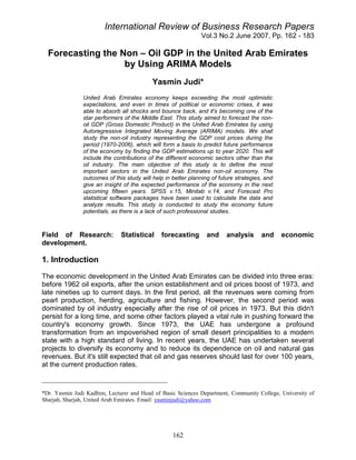
Figure 1: Plot of UAE's non-oil GDP in Millions of USD
From the plot, we see that the production varies considerably. The series wanders tell
us that it is not stationary. In other words, the short term mean level is not constant but
varies over the course of the series. It has also been observed from the plot that short-
term variation also increases or decreases with time. So it is a non-stationary series.
The non-stationary behavior of the series is also confirmed by the estimated ACF of the
series. We find that the ACF dies out slowly confirming the earlier observation that it's
non-stationary. To reach stationary we have taken differencing, as practiced, in
developing ARIMA model.
167
7. Judi
Autocorrelation Function for UAE's non-oil GDP
1.0
0.8
0.6
0.4
Autocorrelation
0.2
0.0
-0.2
-0.4
-0.6
-0.8
-1.0
1 2 3 4 5 6 7 8 9 10 11 12 13 14 15
Lag
Figure 2: ACF for non-oil GDP
From the plot Figure (3) of the difference series in the estimation period, we see that the
mean and variance do not remain constant throughout the production periods indicating
the non-stationary of the production series.
168
9. Judi
This is also supported by ACF of the series Figure (4).
Autocorrelation Function after taking the Difference
1.0
0.8
0.6
0.4
Autocorrelation
0.2
0.0
-0.2
-0.4
-0.6
-0.8
-1.0
1 2 3 4 5 6 7 8 9 10 11 12 13 14 15
Lag
Figure 4: ACF for non-oil GDP after taking the 1st Difference
From the plot Figure (5) of the differenced series in the estimation period, we see that
the mean of the differenced series is about zero from the beginning to the end and the
variance does not noticeably change indicating that the series has attained the
stationary. The ACF of the differenced series figure (6) also confirms this. So the value
of the parameter d of the ARIMA model has been determined and equal to two.
170
10. Judi
Non-oil GDP
5000.00
2500.00
VAR00025
0.00
-2500.00
-5000.00
1970 1972 1974 1976 1978 1980 1982 1984 1986 1988 1990 1992 1994 1996 1998 2000 2002 2004 2006
Years
Figure 5: non-GDP Plot after taking the 2nd Difference
Now to fix the value of p and q of the ARIMA model, we have to study the shape of the
ACF and PACF (partial ACF) of the difference of the series. From the plots Figure (6)
and (7), and we can see that in the ACF.
171
11. Judi
Autocorrelation Function after taking the 2nd Difference
1.0
0.8
0.6
0.4
Autocorrelation
0.2
0.0
-0.2
-0.4
-0.6
-0.8
-1.0
1 2 3 4 5 6 7 8 9 10 11 12 13 14 15
Lag
Figure 6: ACF for non-oil GDP after taking the 2nd Difference
Partial Autocorrelation Function after taking the 2nd Difference
1.0
0.8
0.6
Partial Autocorrelation
0.4
0.2
0.0
-0.2
-0.4
-0.6
-0.8
-1.0
1 2 3 4 5 6 7 8 9
Lag
Figure 7: PACF for non-oil GDP after taking the 2nd Difference
172
12. Judi
From Figure: (6), we also notice that the ACF of the differenced series now dies out
quickly confirming that the stationary of the series has been obtained and hence
provides us the value of the parameter d = 2 of ARIMA model.
Next to identify the value of the other two parameters p and q of ARIMA model, we
study the appearance of the ACF and PACF of the differenced series and Comparing
the two plots given in Figure (6) and (7) we see that there is an unexpected peak in both
the ACF and PACF at lag 1 which can not be explained properly. Aside from the peak
both AR and MA components. Since the series has been differenced for the ACF and
PACF so a mixed ARIMA (0,2,1) for the series may be recommended.
Since the estimated ACF and PACF of the differenced series are quite complex and
identification of ARIMA (0,2,1) is not straight forward and certain so well as, the ARIMA
(0,2,1), there fore we have also fitted other models such as ARIMA (1,2,1), ARIMA
(1,2,0) and compared than with each other before finally accepting any model for the
production series.
4.2 Estimating the Models:
Table (1) shows the estimation of the above-mentioned models selected for the series.
Comparing the results we see that among all fitted models the value R² of ARIMA
(0,2,1) is the highest (R² = 0.98). It is very important to increase confidence of accepted
ِ
model andِadj R²=0.97. This model is explains 97% percentage of the variables of GDP
non-oil. This affected spread values of GDP and sequence forecasting .
The estimates of MAD, MAPE, BIC, RMSE and forecast error are the smallest. The
estimated coefficients of parameters of ARIMA (0,2,1) are found statistically significant
but the estimated coefficients of parameters of the other mentioned models are non-
significant. It is also observed that adding more parameter to ARIMA (1,2,3),(1,2,0)
manifests itself in non-significant coefficient and larger MAPE and BIC values indicate
overfitting of the model. So these over fitted models have been dropped from analysis.
So ARIMA (0,2,1) has been identified as the best production model.
173
13. Judi
ARIMA 0,2,1 1,2,3 1,2,0
R² 0,98 0,98 0,97
Durbin-Watson 2.014 1.994 1.854
Forecast error 1347 1348 1402
MAPE 0.0963 0.117 0.099
5 7 67
MAD 807.5 832.1 892.7
Standard 9332 9332 9332
Deviation
Adjust R² 0.98 0.97 0.97
Ljuny-Box (18) 12.44 12.41 12.16
BIC 1404 1442 1461
RMSE 1323 1380 1376
Table 1: Estimation of the three models
4.3 Diagnosing the Final Model: (The Residual Analysis)
The universal rule for residuals generated by an appropriate model should be randomly
distributed without any pattern (white noise). The plot Figure (8) of residuals created by
ARIMA (0,2,1) show no pattern indicating the appropriateness of the model although a
large outliner is still present.
174
14. Judi
Residual Plots for non-oil GDP
Normal Probability Plot of the Residuals Residuals Versus the Fitted Values
99 5000
90 2500
Residual
Percent
50 0
10 -2500
1 -5000
-5000 -2500 0 2500 5000 0 20000 40000 60000 80000
Residual Fitted Value
Histogram of the Residuals Residuals Versus the Order of the Data
16 5000
12 2500
Frequency
Residual
8 0
4 -2500
0 -5000
-4000 -2000 0 2000 4000 1 5 10 15 20 25 30 35
Residual Observation Order
Figure 8: Plot of ARIMA Model (0,2,1) Residuals
From the ACF and PACF plots of residuals figure (9), (10) we observe that the ACF and
PACF are randomly distributed. All the Box-Ljung Q statistics for the ACF are not
statistically significant at any lag. All these findings further confirm that the residuals are
white noise.
ACF of Residuals for non-oil GDP
1.0
0.8
0.6
0.4
Autocorrelation
0.2
0.0
-0.2
-0.4
-0.6
-0.8
-1.0
1 2 3 4 5 6 7 8 9
Lag
Figure 9: ACF of ARIMA Model (0,2,1) Residuals
175
15. Judi
PACF of Residuals for non-oil GDP
1.0
0.8
Partial Autocorrelation 0.6
0.4
0.2
0.0
-0.2
-0.4
-0.6
-0.8
-1.0
1 2 3 4 5 6 7 8 9
Lag
Figure 10: PACF of ARIMA Model (0,2,1) Residuals
The value of DW statistic is 2.014, which also indicates the absence of first order auto
correlation in the residuals. Moreover from table (2). We also observe that in both the
estimation and predict periods the RMS for residuals created by ARIMA (0,2,1) are the
smallest compared to RMS for residuals created by any other attempted model. This
indicates that the ARIMA (0,2,1) not only fits the data better than any other model but
also reveals that the forecasts based on the model are more accurate. Again, the
normal probability plot Figure (11) of residuals generated by ARIMA (0,2,1) shows that
residuals are approximately follow normal distribution.
So ARIMA (0,2,1) is the appropriate model.
Figure 12: The normal probability of residuals
176
16. Judi
Comparing Box-Jenkins method ARIMA (0, 2, 1) with exponential smoothing and
moving Average methods:
If we examine Figure (1), we can see that the series is too short to be considered for
Box-Jenkins (ARIMA) classical. Now we compare Box-junkies method with exponential
smoothing and moving average methods.
Box-junkies
Moving Exponential
Methods ARIMA
Average smoothing
(0,2,1)
R² 0,98 0.9621 0.979
Durbin-
2.014 0.7316 1.873
Watson
Forecast error 1347 1753 1378
MAPE 0.09635 0.1408 0.1517
MAD 807.5 1254 932.5
Standard
9332 9332 9332
deviation
Adjust R² 0.98 0.9647 0.9782
Ljuny-Box
12.44 7.15 12.28
(18)
BIC 1404 1681 1496
RMSE 1323 1784 1328
Table 2
From Table (1), we can see that the value of adj. R² of ARIMA (0,2,1) is the highest (R²
= 0.98), and it is very important to increase confidence of accepted model.
The estimates of MAD, MAPE, BIC, RMSE and forecast errors are the smallest. The
value of DW statistic is 2.014, which also indicate the absence of first order auto
correlation in the residuals. Moreover, from table (2) we also observe that the value of
RMS (the root mean square error) for residuals created by ARIMA (0,2,1) is the smallest
than RMS for residuals created by any other attempted methods. This indicates that the
ARIMA (0,2,1) is better than any other methods So ARIMA (0,2,1) is the appropriate
model.
After the detailed analysis we notice that the progress of the economy in accordance
with the United Arab Emirates economy during the period from (1970-2006). We have to
put futuristic view that can be drowning in accordance with the economy to the year
(2020), through certain limits, based on the present compared too past.
177
17. Judi
From table (3) we see the result of forecasting.
Period Forecast Lower Upper
2007 83937 78699 89175
2008 88916 81713 96119
2009 94019 84777 103260
2010 99245 87870 110620
2011 104595 90983 118206
2012 110068 94116 126021
2013 115666 97269 134063
2014 121387 100444 142330
2015 127232 103645 150819
2016 133201 106874 159528
2017 139293 110134 168453
2018 145510 113426 177593
2019 151850 116754 186945
2020 158313 120119 196507
Table 3: The result of forecasting of non-oil GDP in UAE (In Millions of USD)
178
18. Judi
Forecasting of UAE's non-oil GDP by using ARIMA (0,2,1)
250,000
200,000
non-oil GDP in Millions of USD
150,000
Actual Values
Predicted Values
Lower Limit
100,000 Upper Limit
50,000
0
1970 1975 1980 1985 1990 1995 2000 2005 2010 2015 2020
Years
Figure 12: Predicted values of UAE's non-oil GDP using the model ARIMA (0,2,1)
From the table and figure above we have reached to the conclusion that non-oil GDP
might probably reach the value of 158313 million USD in 2020 at least. The non-oil GDP
in UAE ranges from a minimum of 120119 million USD limit confidence 95%. We expect
a growing gape between the oil and non-oil economy, for the benefit of increasing
percentage of the contribution of non-oil economy sector. The figure of the minimum
rang which accordingly the non-oil GDP developed shows that in the worst
circumstances the period of year 2006 and till year 2020 will not observe non-oil GDP
less than 120119 million USD.
5. Recommendations:
Emphasize more focus on the non-oil sector, and this will reduce the tendency on
the oil revenue, as the oil is a depleted wealth.
Redistribution of the labor force through the production sectors and the rebuild of
the production environment for other economic sectors that leads to fall and
efficient utilization of labor force.
Reduction of foreign labor force by increasing the motivation and creating
encouragement work atmosphere for the national labor force by adding specific
and plant emigration policy in order to obtain administration and technology.
179
19. Judi
We suggest that the decision-makers have to take a look at the results of this
study, and they should be taken into consideration in forming economic policies.
References
[Abraham, “Statistical Methods for Forecasting”, Second Edition, John Wiley and sons,
N.Y 1983.
Ahmed Abada, Sad Aldin “Introduction applied statistical” printed in Cairo 1972.
Akaike, H.“Maximum Likelihood Identification of Gaussian Autoregressive Regression
Moving Average Models”, Biometrika 60, 255-266, 1973.
Andersion, T.W, “The Statistical Analysis of Time Series”, Second Edition, John Wiley
and Sons, N.Y 1976.
[8] Baker, B.D. "Can Flexible Non-Linear Modeling Tell Us Any thing new about
Education Production", Economics of Education Review, 2001.
Bailey, “The Element of Statistic Processes with Application to the Natural Senesces”,
John Wiley, N.Y, 1964.
Barnett, V and T Lewis, “Outliers in Statistical Data”, Second Edition, John Wiley and
sons, New York 1996.
Bernard ostle, “statistics in Research Basic concepts and Techniques for Research
worker”, Third Edition, printing in 1958.
Bhat, “The Elements of Applied Stochastic Processes”, John Wiley and Sons, New York
1984.
Box, G.E.P and G.M Jenkins, “Time series Analysis forecasting and control”, San
Francisco, Holden Day 1970.
Box, G.E.P. and G.M Ljung on a “Measure of Lack of Fit in Time Series Models”,
Biometrika 65,297-303 in 1978.
Brandt, “Stationary Stochastic Models”, John Wiley and Sons, N.Y.
Brown, R.G. Smoothing, “Forecasting and Prediction of Discrete Time series”,
Englewood Eliffs, N. J. Prentice Hall.
Bruce L. Bowerman and Richard T. O’Connel, “Time series and forecasting” An applied
Approach, printed in U.S.A 1979.
180
20. Judi
C. Chatfield, “The Analysis of Time Series”, Second Edition, Chapman and Hall,
London, 1980.
Chris Chatfield , "The Analysis of Time Series", 6th Edition, Chapman & Hall, 2003.
[16] Cox, D. R. and H. D. Miller, “The Theory of Stochastic Processes”, Chapman and
Hall, London in 1965.
[17] Durbin, J. and G. S. Watson, “Test for Serial Correlation in Least-Squares
Regression”, Biometrika in 1971.
E. J. Hannah “Multiple Time series” John Wiley and sons. Inc. 1970.
Ghosh, Sukesh. Econometrics “Theory and Application”, New Jersey, Prentice Hall
1991.
Granger, C.W and p. Newbold. “Forecasting Economic Time Series”, New York,
Academic press 1986.
Graner, C. W. J. “Forecasting in Business and Economics” Newark Academic press
1989.
[22] Graham Bannock, R.E: Baxter and Evan Davis. The penguim “dictionary of
economics” New Edition 1992.
G – L. Thirkettle, Macdonald and Evan “Welder’s Business statistic” seventh Edition.
London 1977.
Hald, “Statistical Theory with Engineering Application”, (Kolmogorvo-Smirnove Test),
John Wiley, New York in 1952.
Hanan, E. J. “Time Series Analysis”, London, Methuen in 1960.
Hannan, E. J. “Multiple Time Series”, Wiley and Sons, N. Y in 1970.
Harry H – Collegian “Introduction to Econometrics” principles and Applications Second
Edition – Wallace E – oat’s 1981.
-J.Johnston “Econometric Methods” second Edition 1972.
John E-freund and frank J-Williams “Modern Business statistics” printed in Great Britain
1984.
James Douglas Hamilton,"Time Series Analysis", Princeton University Press, 1994.
J. C Hoff , "A practical guide to Box-Jenkins forecasting", 1983.
181
21. Judi
Peter J. Brockwell and Richard A. Davis, "Introduction to Time Series and Forecasting",
Robert H. Shumway, "Time Series Analysis and Its Applications", 2nd Edition, Springer,
2006.
Walter Vandaele , " Applied Time Seriest and Box-Jenkins Models", Academic Press,
1983.
182