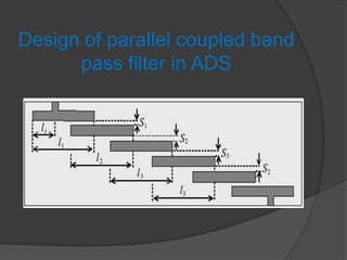
1. Design of parallel coupled band
pass filter in ADS

2. What is an ADS?
 It is an electronic design automation software
system produced by Agilent EEs of EDA, a unit of
Agilent technology.
 More appropriate tool in MHz regime.
 It provides an integrated design environment to
designers of RF electronic products such as
mobile phones, pagers, wireless networks,
satellite communication and etc.
 It provides circuit, 3D electromagnetic field
simulation and offers great flexibility when tackling
SI analysis.
 It has momentum engine which works on moment
technology.

3. Advantages of ADS
 Ease of manufacturing.
 Low fabrication cost.
 Microstrip patch antennas are efficient
radiators.
 It has support for both linear and circular
polarization.
 Easy in integration with microwave integrated
circuits.

4. A parallel coupled bad pass filter was designed in ADS
and simulated.
SUBSTRATE
Bandwidth : 4180 MHz to 4200 MHz
H=50 mil
S21 / S12 <0.5dB Er=10.2
T=35um
S22/S11 <-5 dB in 418 MHz to 4200 MHz and max of -20dB Tan D=0.002
S21 = -35dB to -45 dB at centre frequency ± 350 MHz
Also the design constraints for fabrication are
The minimum width of microstrip line should be 8 mil.
The minimum spacing between two microstrip line should be 10 mil.

5. Schematic design:

6. Substrate characteristics :

7. Final layout of the design:

8. Simulation result

9. The above graph shows
 The centre frequency to be around 4.18
GHz.
 The S21 parameter for centre frequency
±350 MHz is about -35 dB.
 The S21 parameter for centre frequency
is less than 0.5 dB.

10. Testing result:

11. TT&C RF LINK BUDGET

12. Introduction :
 A satellite link is defined as an Earth station -
satellite - Earth station connection. The Earth
station - satellite segment is called the uplink
and the satellite - Earth station segment is
called the downlink.
 The Earth station design consists of the
Transmission Link Design, or Link Budget, and
the Transmission System Design.
 The Link Budget establishes the resources
needed for a given service to achieve the
performance objectives.

13.  The satellite link is composed primarily of
three segments:
 (i) the transmitting Earth station and the
uplink media;
 (ii) the satellite; and
 (iii) the downlink media and the receiving
Earth station.
 The carrier level received at the end of the
link is a straightforward addition of the
losses and gains in the path between
transmitting and receiving Earth stations.

14. Typical satellite link

15. C/N ratio
 The basic carrier-to-noise relationship in a
system establishes the transmission
performance of the RF portion of the system,
and is defined by the receive carrier power level
compared to the noise at the receiver input. For
example, the downlink thermal carrier-to-noise
ratio is:
C/N = C -10log(kTB)
 Where:
 C = Received power in dBW
 k = Boltzman constant, 1.38*10-23 W/°K/Hz
 B = Noise Bandwidth (or Occupied Bandwidth) in Hz
 T = Absolute temperature of the receiving system in °K

16. Link Parameters’ Impact on Service Quality

17. Equivalent Isotropically Radiated
Power:
EIRP is defined as amount of power that a
theoretical isotropic antenna would emit to
produce the peak power density observed in the
direction of maximum antenna gain.
The gain of a directive antenna results in a more
economic use of the RF power supplied by the
source. Thus, the EIRP is expressed as a function
of the antenna transmit gain GT and the
transmitted power PT fed to the antenna.
EIRPdBW = 10 log PT dBw + GT dBi
Where:
PT dBw = antenna input power in dBW
GT dBi = transmit antenna gain in dBi

18. Intermodulation back off
 Because of non linear behavior of TWT
amplifier present in transponder.
 Non linear behavior give rise to
intermediate products and cross-talk.
 In order to improve C/N or reduce this
intermediate products the operating point
shifted to linear part of characteristics.
 This shift can be realized by controlling
ground level EIRP which give rise to
reduction in output power known as output
back off.

19. Antenna Gain
The antenna gain, referred to an isotropic
radiator, is defined by:
GdBi = ηD
Where:
η = antenna efficiency (Typical values are 0.55 - 0.75)
D = Directivity of the antenna
Basically antenna gain has no limit but has to be restricted
due to cost and surface imperfection.

20. Free space path loss
 Free-space path loss (FSPL) is the loss in
signal strength of an electromagnetic wave
that would result from a line-of-sight path
through free space (usually air), with no
obstacles nearby to cause reflection or
diffraction.
Lo = 20log(d) + 20log(f) + 92.5 dB
 It does not include factors such as the gain of
the antennas used at the transmitter and
receiver, nor any loss associated with
hardware imperfections
 It is order of around 200dB.

21. Polarization loss
Polarization loss are non linear losses due to misalignment
b/w transmitter antenna and receiver antenna. Every antenna
radiates its electric field in preferred orientation, and can be
either linear polarized or circularly polarized. Linear fields
aligned in same direction transfer the maximum signal and
while orthogonal gives the least because theoretically there is
no coupling.

22. For linear polarization.
Loss (in DB) = 10*(log base 10)(cos(theta))^2
Where theta is the angle between the
polarization vectors. Therefore, if a vertically
polarized antenna is used to copy a vertically
polarized signal, the loss due to polarization is
zero DB. If they are at 90 degrees, cross
polarized, the loss is infinite

23. Pointing /Tracking Losses
When a satellite link is established, the ideal
situation is to have the Earth station antenna
aligned for maximum gain, but normal operation
shows that there is a small degree of misalignment
which causes the gain to drop by a few tenths of a
dB. The gain reduction can be estimated from the
antenna size, the tracking type, and accuracy.
This loss must be considered for the uplink and
downlink calculations.

24. Earth Station Performance Characteristic (C-band,
Antenna Efficiency 70%)

25. To determine the expected amount of pointing loss, the
design engineer will consider such things as antenna
position, encoder accuracy, resolution of position
commands, and autotrack accuracy. The pointing
accuracy of both the spacecraft antenna and the ground
station antenna must be considered, although they may
both be combined into one entry in the link budget.
Pointing loss will usually be small, on the order of a few
tenths of a dB. This is small enough for the maintenance
engineer to ignore under normal circumstances.
However, pointing loss is one of the most common
causes of link failure. This is usually due to inaccurate
commanded position of the antenna, but can also be
caused by a faulty position encoder.

26. Atmospheric Losses
Losses in the signal can also occur through
absorption by atmospheric gases such as
oxygen and water vapor. This characteristic
depends on the frequency, elevation angle,
altitude above sea level, and absolute humidity.
At frequencies below 10 GHz, the effect of
atmospheric absorption is negligible.
Its importance increases with frequencies above 10
GHz, especially for low elevation angles.

27. Atmospheric Losses
 Table shows an example of the mean value of
atmospheric losses for a 10-degree elevation
angle.

28. Atmospheric Attenuation

29. Atmospheric Absorption
Contributing Factors:
– Molecular oxygen Constant
– Uncondensed water vapor
– Rain
– Fog and clouds Depend on
weather
– Snow and hail
• Effects are frequency dependent
– Molecular oxygen absorption peaks at 60 GHz
– Water molecules peak at 21 GHz
• Decreasing elevation angle will also increase
absorption loss

30. Rain Effects
 An important climatic effect on a satellite link is the
rainfall. Rain results in attenuation of radio waves by
scattering and by absorption of energy from the
wave.
 Rain attenuation increases with the frequency, being
worse for Ku-band than for C-band. Enough extra
power must be transmitted to overcome the
additional attenuation induced by rain to provide
adequate link availability.
 Specified rain fade is typically in range of 6dB.
 Another effect of rain is signal depolarization, causes
increase in polarization loss.

31. Typical Losses

32. System Noise Temperature
The system noise temperature of an Earth station consists
of the receiver noise temperature, the noise temperature
of the antenna, including the feed and waveguides, and
the sky noise picked up by the antenna.
Tsystem = Tant/L + (1 - 1/L)To + Te
Where:
L = feed loss in numerical value
Te= receiver equivalent noise temperature
To= standard temperature of 290°K
Tant = antenna equivalent noise temperature as provided
by the manufacturer

33. Noise Sources
System Noise
– Received power is very small, in picowatts
– Thermal noise from random motion of electrons
– Antenna noise: antenna losses + sky noise (background microwave radiation)
– Amplifier noise temperature: energy absorption manifests itself as heat, thus
generating thermal noise
• Carrier-to-Noise Ratio
– C/N = PR - PN in dB
– PN = k TN BN
– C/N = EIRP + GR - LOSSES - k -TS - BN
where k is Boltzman’s constant, TS is system noise temperature, TN is equivalent
noise temperature, BN is the equivalent noise bandwidth
– Carrier to noise power density (noise power per unit b/w):
C/N0 = EIRP + G/T - Losses - k

34. Antenna Noise Temperature
 The noise power into the receiver, (in this case the LNA),
due to the antenna is equivalent to that produced by a
matched resistor at the LNA input at a physical
temperature of Tant.
 If a body is capable of absorbing radiation, then the body
can generate noise. Thus the atmosphere generates some
noise. This also applies to the Earth surrounding a
receiving ground station antenna. If the main lobe of an
antenna can be brought down to illuminate the ground, the
system noise temperature would increase by
approximately 290°K.

35. Antenna Noise Temperature
Noise Temperature of an Antenna as a Function of Elevation Angle

36. Figure of Merit (G/T)
In every transmission system, noise is a factor that
greatly influences the whole link quality.
The G /TdBK is known as the "goodness"
measurement of a receive system.
This means that providing the Earth station meets
the required G/T specification, INTELSAT will
provide enough power from the satellite to meet the
characteristic of every service.

37. Figure of Merit (G/T)
G/T is expressed in dB relative to 1°K. The same
system reference point, such as the receiver input,
for both the gain and noise temperature must be
used.
G/T = Grx - 10log(Tsys)
Where:
Grx = receive gain in dB
Tsys = system noise temperature in °K

38. Carrier to Noise Ratio
The ratio C/No allow us to compute directly the
receiver Bit energy-to-noise density ratio as:
Eb/No = C/No - 10log(digital rate)
The term "digital rate" is used here because Eb/No
can refer to different points with different rates in
the same modem.

39. Carrier-to-Noise Ratio
Example Calculation
– 12 GHz frequency, free space loss = 206 dB,
antenna pointing loss = 1 dB,
atmospheric absorption = 2 dB
– Receiver G/T = 19.5 dB/K,
receiver feeder loss = 1 dB
– EIRP = 48 dBW
• Calculation:
– C/N0 = -206 - 1 - 2 + 19.5 - 1 + 48 + 228.6 = 86.1
(Note that Boltzmann’s constant k
= 1.38x10-23 J/K = -228.6 dB)