A global approach with cutoff exponential functions is used to obtain the Casimir energy of a massless scalar field in the presence of a spherical shell. The proposed method, mathematically well defined at the outset, makes use of two regulators, one of them to make the sum of the orders of Bessel functions finite and the other to regularize the integral involving the zeros of Bessel function. This procedure ensures a consistent mathematical handling in the calculations of the Casimir energy and allows a major comprehension on the regularization process when nontrivial symmetries are under consideration. In particular, we determine the Casimir energy of a scalar field, showing all kinds of divergences. We consider separately the contributions of the inner and outer regions of a spherical shell and show that the results obtained are in agreement with those known in the literature, and this gives a confirmation for the consistence of the proposed approach. The choice of the scalar field was due to its simplicity in terms of physical quantity spin. Publication Name: Advances in High Energy Physics. Author: M.S.R. Miltão and Franz A. Farias.

1. Hindawi Publishing Corporation
Advances in High Energy Physics
Volume 2010, Article ID 120964, 13 pages
doi:10.1155/2010/120964
Research Article
A Global Approach with Cutoff Exponential
Function, Mathematically Well Defined at
the Outset, for Calculating the Casimir Energy:
The Example of Scalar Field
M. S. R. Milt˜ao and Franz A. Farias
Departamento de F´ısica-UEFS, 44036-900 Feira de Santana, BA, Brazil
Correspondence should be addressed to M.S.R. Milt˜ao, miltaaao@ig.com.br
Received 9 October 2010; Accepted 6 December 2010
Academic Editor: Ira Rothstein
Copyright q 2010 M.S.R. Milt˜ao and F. A. Farias. This is an open access article distributed under
the Creative Commons Attribution License, which permits unrestricted use, distribution, and
reproduction in any medium, provided the original work is properly cited.
A global approach with cutoff exponential functions is used to obtain the Casimir energy of
a massless scalar field in the presence of a spherical shell. The proposed method, mathematically
well defined at the outset, makes use of two regulators, one of them to make the sum of the orders
of Bessel functions finite and the other to regularize the integral involving the zeros of Bessel
function. This procedure ensures a consistent mathematical handling in the calculations of the
Casimir energy and allows a major comprehension on the regularization process when nontrivial
symmetries are under consideration. In particular, we determine the Casimir energy of a scalar
field, showing all kinds of divergences. We consider separately the contributions of the inner
and outer regions of a spherical shell and show that the results obtained are in agreement with
those known in the literature, and this gives a confirmation for the consistence of the proposed
approach. The choice of the scalar field was due to its simplicity in terms of physical quantity
spin.
1. Introduction
The relevance of the Casimir effect has increased over the decades since the seminal paper
1948 1 by the Dutch Physicist Hendrik Casimir. This effect concerns to the appearance of
an attractive force between two plates when they are placed close to each other. Casimir was
the first to predict and explain the effect as a change in vacuum quantum fluctuations of the
electromagnetic field.

2. 2 Advances in High Energy Physics
Nowadays, the Casimir effect has been applied to a variety of quantum fields and
geometries and it has gained a wider understanding as the effect which comes from the
fluctuations of the zero point energy of a relativistic quantum field due to changes in its base
manifold. This interpretation can be confirmed when we see the large range where the
Casimir effect has been applied: the study of gauge fields with BRS symmetry 2 , in the
Higgs fields 3 , in supersymmetric fields 4 , in supergravity theory 5, 6 , in superstrings
7 , in the Maxwell-Chern-Simons fields 8 , in relativistic strings 9 , in M-theory 10 ,
in cosmology 11 , and in noncommutative spacetimes 12 , among other subjects in the
literature 13, 14 , the review articles 15–17 , and textbooks 18–23 .
In this present work, the meaning of base manifold is that the confinement that
the field is subjected is due to the presence of a sphere, where the boundary conditions
take place. The point we aim to emphasize is that once the calculation of the Casimir
effect involves dealing with infinite quantities, we need to use a regularization procedure
appropriately defined. Many different regularization methods have been proposed and we
can quote some of them: the summation mode method—using the general cutoff function
1 , exponential cutoff function 24, 25 , Green function 26–30 , Green function through
multiple scattering 31 , exponential function and cutoff parameter 32, 33 , zeta function
34–40 , Abel-Plana formula 21, 41 , or point-splitting 42–44 ; the Green function method—
using the point-splitting 45–48 , Schwinger’s source theory 49–51 , or zeta function
52 ; the statistical approach method—using the path integral formalism 53 , or Green
function 54 ; as some examples among others. These methods are distinguished by the
approach used to carry out the calculations of the Casimir energy, and it is clear that
the physical result must be independent from the regulators or the method employed for
them. But the literature has shown that the results found there exhibit a divergence among
them.
In a general way, the methods used to obtain the Casimir effect lie on one of the two
categories: a local procedure or a global one. With a local procedure, we mean one that the
expression for the change of the vacuum energy is explicitly dependent on the variables of the
base manifold, and only in the final step of calculations the integration over these variables
is carried out. On the other hand, in a global one, we start with an expression for the vacuum
energy where there is no space-time variables present as they already were integrated.
In the present work, we pretend detailing a global approach 55, 56 for the calculation
of Casimir energy. In this method, mathematically well defined at the outset, we propose
the use of two regulators into the cutoff exponential function, and we demonstrate that this
regularization approach is one appropriate for the calculation of Casimir effect in the case of
nontrivial symmetries, in particular a spherical symmetry.
With the use of scalar field, we can avoid the inherent complications brought by the
vector nature of the electromagnetic field, and due to its simple structure, the scalar field
usually becomes an effective tool to be used in the investigation of field proprieties as in these
examples: in the dynamical Casimir effect 57 , in the Casimir effect at finite temperature
58, 59 , and in the Casimir effect on a presence of a gravitational field 60, 61 , among others
62–64 .
The paper is organized as follows: we detail in Section 2 the method to be used and
why we need two cutoff parameters to obtain an regularized expression for the Casimir
energy, which is the starting point for a consistent mathematical handling. Section 3 exhibits
the calculations for the contributions of the inner and the outer regions of the spherical shell.
We analyze in Section 4 the results and compare them with those ones in the literature and
make some considerations.

3. Advances in High Energy Physics 3
2. The Global Procedure Proposed with Two Parameters
The starting point is the expression for the Casimir energy defined as the difference between
the vacuum energy under a given boundary condition and the reference vacuum energy.
When we consider a scalar field in the presence of a spherical shell, this vacuum energy is
E0
∞
n 1
∞
j 0
j
m −j τ
1
2
ωτ
jn, 2.1
where ωτ
jn are the mode frequencies. They are obtained when the boundary conditions are
imposed on the field. In the absence of boundary conditions, the frequencies take some values
which let us designate as ω
τ ref
jn and these lead to the vacuum reference energy
E ref
∞
n 1
∞
j 0
j
m −j τ
1
2
ω
τ ref
jn , 2.2
so the Casimir energy is E E0 − E ref
. The boundary conditions due to a spherical shell with
radius a are
kajj ka 0, for r a − 0,
Ajkajj ka Bj kanj ka 0, for r a 0.
2.3
The Casimir energy will be calculated by using the mode summation and the argument
theorem also known as argument principle 65–67 . This theorem gives the summation of
zeros and poles of an analytic function as a contour integral. This contour is a curve that
encompasses the interior region of the complex plane which contains the zeros and poles
65–67 . In our case, we are interested in the root functions which match the conditions 2.3 .
So, the following equations are appropriate as root functions
f1
j az azjj az ,
f2
j az cos δj z azjj az tan δj z aznj az ,
2.4
where
z k
ω
c
, δj z zR −
jπ
2
. 2.5
When we apply the argument theorem and carry out some handling, we get
g
n 1
ωτ
jn
c
2πi C
dz z
d
dz
log fτ
j az . 2.6

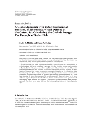
4. 4 Advances in High Energy Physics
ϕ
Γ1
Γ2
ϕ Cλ
Figure 1: The path of integration in the complex plane.
a
R
R/ξ
R
Figure 2: A sketch of the subtraction process which takes place on the regularization of the Casimir effect
of a spherical shell.
In the above equation, the argument for logarithm must involve the product of all root
functions. The contour to be taken on the calculations is given by 68 according to Figure 1.
The subtraction process renormalization , defined by E, can be schematically
represented as in Figure 2.
The vacuum energy 2.1 which takes into account the boundary conditions can be
used to obtain the reference energy in 2.2 . This is done when we take the limit for the
radius a going to infinity. This procedure is sensible, but it already has been made clear by
Boyer 69, 70 . After all, we obtain for the Casimir energy
E
∞
n 1
∞
j 0
j
m −j
4
τ 1
1
2
ωτ
jn − ω
τ ref
jn
lim
σ → 0, → 0, R → ∞, ξ → 1
c
2πi
∞
j 0
ν exp − ν
C
dz z exp −σz
×
d
dz
log f
1
j az f
2
j az − log f
1 ref
j
R
ξ
z f
2 ref
j
R
ξ
z ,
2.7

5. Advances in High Energy Physics 5
where ν j 1/2. We can see from above that two exponential functions were used, one of
them is the function under the integral sign, exp −σz , σ > 0 , that stems from the argument
theorem and the other is the function exp − ν , > 0 , under summation sign on j ν −
1/2 . Now, group together these two developments, and 2.7 may be rewritten as
E −
c
π
Ê
∞
j 0
ν2
exp − ν
∞ exp −iϕ
0
dz exp −iσνz z
d
dz
log Iν νaz log Kν νaz
− E ref
,
2.8
where the limits for R and ξ have been taken into account. The other limits will be taken in
an appropriate moment after the cancelation of possible remaining divergences.
3. Casimir Effect of a Spherical Shell: The Case of a Scalar Field
We now rewrite 2.8 in a more appropriate way, so that the contributions can be separated
by regions as E EI EO, where
EI −
c
π
Ê 1
2
2
exp −
1
2
∞ exp −iϕ
0
dz z exp −iσ
1
2
z
d
dz
log I1/2
1
2
az
−
c
π
Ê
∞
j 1
ν2
exp − ν
∞ exp −iϕ
0
dz z exp −iσνz
d
dz
log Iν νaz − Eref
I
3.1
is the contribution due to the internal modes and
EO −
c
π
Ê 1
2
2
exp −
1
2
∞ exp −iϕ
0
dz z exp −iσ
1
2
z
d
dz
log K1/2
1
2
az
−
c
π
Ê
∞
j 1
ν2
exp − ν
∞ exp −iϕ
0
dz z exp −iσνz
d
dz
log Kν νaz − Eref
O
3.2
is the contribution due to the external modes. As it can be observed, the above contributions
were written in such a way that the term for j 0 was detached from the summation on j.
This has been done to the effect of making explicit the term on which we will focus attention
as well as taking into account some developments already accomplished 55 .
3.1. Internal Mode
Now, we proceed with the calculations of 3.1 , and the first step is to take the Debye
expansion for the Bessel functions up to order O ν−4
71, 72 . The Debye expansion gives

6. 6 Advances in High Energy Physics
accurate results when we consider large order of ν j 1/2 and larger arguments and that
also makes an analytical treatment possible for the resulting expressions. So, we have
EI EI − E
ref
I , 3.3
where EI EI,0 EI,1 EI,2 EI,3 EI,4 and the terms EI,n are given by
EI,0 −
c
2π
Êexp −
1
2
exp −iϕ
∞
0
dρ exp −iσρ exp −iϕ
× −
1
2
exp −iϕ aρ coth aρ exp −iϕ ,
3.4
EI,1
c
πa
∞
j 1
ν2
∞
0
dρ log II ν, ρ −
4
k 1
U I,k t
νk
, 3.5
EI,2 −
c
π
Ê
4
k 1
∞
j 1
ν2−k
exp − ν
∞ exp −iϕ
0
dz exp −iσνz z
d
dz
U I,k t , 3.6
EI,3
c
2π
Ê
∞
j 1
ν2
exp − ν
∞ exp −iϕ
0
dz exp −iσνz
a2
z2
1 a2z2
, 3.7
EI,4 −
c
π
Ê
∞
j 1
ν3
exp − ν
∞ exp −iϕ
0
dz exp −iσνz 1 a2z2, 3.8
with the definitions 37
II ν, ρ
√
2πν 1 ρ2
1/4
exp −νη Iν νρ , 3.9
U I,1 t
t
8
−
5t3
24
, 3.10
U I,2 t
t2
16
−
3t4
8
5t6
16
, 3.11
U I,3 t
25t3
384
−
531t5
640
221t7
128
−
1105t9
1152
, 3.12
U I,4 t
13t4
128
−
71t6
32
531t8
64
−
339t10
32
565t12
128
. 3.13
The contributions 3.7 and 3.8 compound the zero-order terms of the Debye expansion.
The contribution 3.5 stems from small values of the angular momentum j, and its value
was already determined by 37
EI,1 0.00024
c
πa
. 3.14

7. Advances in High Energy Physics 7
The contributions 3.6 to 3.8 are calculated taking into account the Euler-Maclaurin
formula with remainder 73–75 , and these were calculated by 55
EI,2
c
π
Ê 8099
63839
1
a
7
24
a
σ2
11
192
1
a
log
σ
a
229
40320
1
a
log i
7801
86684
1
a
, 3.15
EI,3
c
π
Ê 52529
267528
1
a
i −
1
3
1
σ
−
3
4
1
σ
−
1
2
1
σ 2
, 3.16
EI,4
c
π
Ê 7375
85696
1
a
−
11
24
a
σ2
2
a3
σ4
−
127
1920
1
a
log
σ
a
− i
2197
21145
1
a
. 3.17
Collecting the terms 3.14 , 3.15 , 3.16 , and 3.17 , we get
EIpartial
0.4095155894
c
πa
c
π
−
1
6
a
σ2
2
a3
σ4
−
17
1920
1
a
log
σ
a
229
40320
1
a
log . 3.18
For 3.4 , corresponding to j 0, we obtain
EI,0
c
π
−
1
24
π2
a
1
2
a
σ2
. 3.19
So, the energy of a scalar field considering a spherical configuration due the internal modes
is
EI EIpartial
EI,0
−
c
πa
0.0017179275
c
π
1
3
a
σ2
2
a3
σ4
−
17
1920
1
a
log
σ
a
229
40320
1
a
log .
3.20
The expression 3.20 shows in an undoubted way the need for a second regularized
exponential function, exp − ν , to make a consistent mathematical handling of the
divergences possible. Both divergences, the logarithm in 3.15 and the polynomial in 3.16 ,
stem from the summation on j. This type of divergence was already observed in 76 , but
only with the procedure established here this discard turns to be completely justified as an
appropriate regularization allows the real part of 3.16 to be taken in an unambiguous way.
3.2. External Mode
The contribution of the external modes comes by 3.2 . We proceed with the calculations in
an analogous way to that of the previous subsection. So,
EO EO − E
ref
O , 3.21

8. 8 Advances in High Energy Physics
where EO EO,0 EO,1 EO,2 EO,3 EO,4 and
EO,0 −
c
2π
Êexp −
1
2
exp −iϕ
∞
0
dρ exp −iσρ exp −iϕ −
1
2
− exp −iϕ aρ , 3.22
EO,1
c
πa
∞
j 1
ν2
∞
0
dρ log KO ν, ρ −
4
k 1
U O,k t
νk
, 3.23
E0,2 −
c
π
Ê
4
k 1
∞
j 1
ν2−k
exp − ν
∞ exp −iϕ
0
dz exp −iσνz z
d
dz
U O,k t , 3.24
EO,3
c
2π
Ê
∞
j 1
ν2
exp − ν
∞ exp −iϕ
0
dz exp −iσνz
a2
z2
1 a2z2
, 3.25
EO,4
c
π
Ê
∞
j 1
ν3
exp − ν
∞ exp −iϕ
0
dz exp −iσνz 1 a2z2, 3.26
with the following definitions 37 :
KO ν, ρ
2ν
π
1 ρ2
1/4
exp νη Kν νρ , 3.27
U O,1 t −U I,1 t , 3.28
U O,2 t U I,2 t , 3.29
U O,3 t −U I,3 t , 3.30
U O,4 t U I,4 t , 3.31
where the U O,k are given by 3.10 to 3.13 , respectively. The term 3.28 was numerically
determined by 37
EO,1 −0.00054
c
πa
. 3.32
The other contributions are calculated following the analogous procedure detailed in the
previous subsection:
EO,2
c
π
Ê −
5821
56688
1
a
−
7
24
a
σ2
−
11
192
1
a
log
σ
a
−
229
40320
1
a
log − i
7801
86684
1
a
,
EO,3 EI,3,
EO,4 −EI,4 .
3.33

9. Advances in High Energy Physics 9
After collecting the terms 3.32 and 3.33 , we have
EOpartial
0.01056399145
c
πa
c
π
1
6
a
σ2
− 2
a3
σ4
17
1920
1
a
log
σ
a
−
229
40320
1
a
log . 3.34
The contribution 3.22 , related to j 0, when we repeat the calculation gives
EO,0
c
π
−
1
2
a
σ2
. 3.35
Gathering together 3.34 and 3.35 , we get the total contribution to the energy of a scalar
field of a spherical configuration due the external modes
EO EOpartial
EO,0
c
πa
0.01056399145
c
π
−
1
3
a
σ2
− 2
a3
σ4
17
1920
1
a
log
σ
a
−
229
40320
1
a
log .
3.36
Our next task is to determine the reference energy and take the regularizations as indicated
by 3.3 and 3.21 .
4. The Regularized Results
Calculating the reference energy, we get
E
ref
± ±
R
ξ
f
σ2
, 4.1
where the plus sign refers to EI and the minus sign to EO and
f exp −
2
3 exp − 1 exp − 1
−2
. 4.2
Now, we can gather together the internal 3.20 and external 3.36 contributions,
taking into account 4.1 , to obtain the Casimir effect for a scalar field due to the presence
of a spherical shell with radius a
E a
c
a
0.002815789609. 4.3
This result is free of divergences since we get an exact cancelation for the terms which depend
on the cutoff parameters. Equation 4.3 is in agreement with that obtained by 37 , through
the zeta function method, and with that in 77 , which uses the Green function formalism and
the dimensional analytical extension in this reference the starting point is the expression for
the force .

10. 10 Advances in High Energy Physics
5. Conclusions
Our purpose in this work was to show the form and nature of each divergent term that
appears in the calculation of Casimir energy and demonstrate that the method proposed is
mathematically consistent and that it is in accordance with the results existing in literature.
To this end, we show explicitly, to the scalar field, the characteristic of the divergent
terms calculated in 3.20 , 3.36 , and 4.1 as a function of the geometrical proprieties of
boundary if we rewrite the divergent part of those assuming a dimensionless parameter ε
a 357/155
, with dim L−1
, so
E± ± c
3
π2
V a
1
σ4
−
17
3840π2
S a κ3
log σε
1
3π2
S a κ
1
σ2
−
1
4π2
S
R
ξ
κS
R
ξ
f ε
σ2
,
5.1
where the plus sign refers to the index I while the minus sign refers to the index O, and
κ 1/a is the curvature. In 5.1 , V a is a volume, S a is an area, and σ and are cutoff
parameters. As we can see, the second and fourth terms in 5.1 explain why two regulators
are required to get a well-defined expression for the Casimir energy of the scalar field. This
is the same case when we consider an electromagnetic field see 55 . The result 5.1 is in
agreement with 78 , except for the divergence due to log and due to the relative self-
energy of the spherical shell, f ε /σ2
, that does not appear there.
Our purpose in this work is to confirm that the prescription in 2.7 works well
when we assume non trivial symmetries for the fields. In fact, the approach has succeed
in demonstrating the cancelation of all types of divergences appearing in the expression for
the Casimir energy of the scalar field. Besides, this calculation presented at this work shows
the desired agreement with the results existing in the literature. Furthermore, as it has been
mentioned by the authors in 79–81 , a better understanding of the quantum field theory
undoubtedly involves the necessity to understand these infinities.
Acknowledgment
The authors wish to thank Dr. Ludmila Oliveira H. Cavalcante DEDU-UEFS for valuable
help with English revision.
References
1 H. B. G. Casimir, “On the attraction between two perfectly conducting plates,” Proceedings of the Royal
Netherlands Academy of Arts and Sciences, vol. 51, pp. 793–795, 1984.
2 J. Ambjørn and R. J. Hughes, “Gauge fields, BRS symmetry and the Casimir effect,” Nuclear Physics
B, vol. 217, no. 2, pp. 336–348, 1983.
3 H. Aoyama, “Casimir energy of Higgs-field configurations in a Coleman-Weinberg-type theory,”
Physical Review D, vol. 29, no. 8, pp. 1763–1771, 1984.
4 Y. Igarashi, “Supersymmetry and the Casimir effect between plates,” Physical Review. D, vol. 30, no. 8,
pp. 1812–1820, 1984.
5 T. Inami and K. Yamagishi, “Vanishing quantum vacuum energy in leven-dimensional supergravity
on the round seven-sphere,” Physics Letters B, vol. 143, no. 1–3, pp. 115–120, 1984.
6 K. Kikkawa, T. Kubota, S. Sawada, and M. Yamasaki, “Stability of self-consistent dimensional
reduction,” Physics Letters B, vol. 144, no. 5-6, pp. 365–369, 1984.
7 K. Kikkawa and M. Yamasaki, “Casimir effects in superstring theories,” Physics Letters B, vol. 149, no.
4-5, pp. 357–360, 1984.

11. Advances in High Energy Physics 11
8 K. A. Milton and Y. J. Ng, “Maxwell-chern-simons Casimir effect,” Physical Review D, vol. 42, no. 8,
pp. 2875–2880, 1990.
9 I. Brevik and R. Sollie, “On the Casimir energy for a 2N-piece relativistic string,” Journal of
Mathematical Physics, vol. 38, no. 6, pp. 2774–2785, 1997.
10 M. Fabinger and P. Hoˇrava, “Casimir effect between world-branes in heterotic M-theory,” Nuclear
Physics. B, vol. 580, no. 1-2, pp. 243–263, 2000.
11 S. Nojiri, S. D. Odintsov, and S. Zerbini, “Bulk versus boundary gravitational Casimir effects in the
quantum creation of an inflationary brane-world universe,” Classical and Quantum Gravity, vol. 17, no.
23, pp. 4855–4866, 2000.
12 M. Demetrian, “Casimir effect in four simple situations—including a noncommutative two-sphere,”
Fizika B, vol. 11, pp. 175–190, 2002.
13 G. J. Maclay, H. Fearn, and P. W. Milonni, “Of some theoretical significance: implications of Casimir
effects,” European Journal of Physics, vol. 22, no. 4, pp. 463–469, 2001.
14 M. S. R. Milt˜ao, Estudo do Efeito Casimir Eletromagn´etico Esf´erico pelo M´etodo da Dupla Regularizac¸˜ao, Tese
de Doutorado, Universidade Federal do Rio de Janeiro, 2004.
15 G. Plunien, B. M¨uller, and W. Greiner, “The Casimir effect,” Physics Reports, vol. 134, no. 2-3, pp.
87–193, 1986.
16 S. K. Lamoreaux, “Resource letter CF-1: Casimir force,” American Journal of Physics, vol. 67, no. 10, pp.
850–861, 1998.
17 M. Bordag, U. Mohideen, and V. M. Mostepanenko, “New developments in the Casimir effect,”
Physics Reports, vol. 353, no. 1-3, pp. 1–205, 2001.
18 P. W. Milonni, The Quantum Vacuum: An Introduction to Quantum Electrodynamics, Academic Press,
Boston, Mass, USA, 1994.
19 E. Elizalde, S. D. Odintsov, A. Romeo, A. A. Bytsenko, and S. Zerbini, Zeta Regularization Techniques
with Applications, World Scientific Publishing, River Edge, NJ, USA, 1994.
20 E. Elizalde, Ten Physical Applications of Spectral Zeta Functions, Springer, Berlin, Germany, 1995.
21 V. M. Mostepanenko and N. N. Trunov, The Casimir Effect and Its Applications, Clarendon Press, Oxford,
UK, 1997.
22 K. A. Milton, The Casimir Effect, World Scientific Publishing, River Edge, NJ, USA, 2001.
23 M. Bordag, G. L. Klimchitskaya, U. Mohideen, and V. M. Mostepanenko, Advances in the Casimir Effect,
Oxford University Press, New York, NY, USA, 2009.
24 B. Davies, “Quantum electromagnetic zero-point energy of a conducting spherical shell,” Journal of
Mathematical Physics, vol. 13, p. 1324, 1972.
25 T. H. Boyer, “Quantum electromagnetic zero-point energy of a conducting spherical shell and the
casimir model for a charged particle,” Physical Review, vol. 174, no. 5, pp. 1764–1776, 1968.
26 W. Lukosz, “Electromagnetic zero-point energy shift induced by conducting closed surfaces,”
Zeitschrift f¨ur Physik, vol. 258, no. 2, pp. 99–107, 1973.
27 W. Lukosz, “Electromagnetic zero-point energy shift induced by conducting surfaces—II. The infinite
wedge and the rectangular cavity,” Zeitschrift f¨ur Physik, vol. 262, no. 4, pp. 327–348, 1973.
28 C. M. Bender and P. Hays, “Zero-point energy of fields in a finite volume,” Physical Review D, vol. 14,
no. 10, pp. 2622–2632, 1976.
29 Siddhartha Sen, “A calculation of the Casimir force on a circular boundary,” Journal of Mathematical
Physics, vol. 22, no. 12, pp. 2968–2973, 1981.
30 J. Baacke and Y. Igarashi, “Casimir energy of confined massive quarks,” Physical Review D, vol. 27, no.
2, pp. 460–463, 1983.
31 R. Balian and B. Duplantier, “Electromagnetic waves near perfect conductors. II. Casimir effect,”
Annals of Physics, vol. 112, no. 1, pp. 165–208, 1978.
32 K. Olaussen and F. Ravndal, “Electromagnetic vacuum fields in a spherical cavity,” Nuclear Physics,
Section B, vol. 192, no. 1, pp. 237–258, 1981.
33 K. Olaussen and F. Ravndal, “Chromomagnetic vacuum fields in a spherical bag,” Physics Letters B,
vol. 100, no. 6, pp. 497–499, 1981.
34 J. R. Ruggiero, A. H. Zimerman, and A. Villani, “Application of analitical regularization to the Casimir
forces,” Revista Brasileira de F´ısica, vol. 7, p. 663, 1977.
35 S. W. Hawking, “Zeta function regularization of path integrals in curved spacetime,” Communications
in Mathematical Physics, vol. 55, no. 2, pp. 133–148, 1977.
36 M. Bordag, E. Elizalde, and K. Kirsten, “Heat kernel coefficients of the Laplace operator on the D-
dimensional ball,” Journal of Mathematical Physics, vol. 37, no. 2, pp. 895–916, 1996.

12. 12 Advances in High Energy Physics
37 S. Leseduarte and August Romeo, “Complete zeta-function approach to the electromagnetic Casimir
effect for spheres and circles,” Annals of Physics, vol. 250, no. 2, pp. 448–484, 1996.
38 N. Shtykovt and D. V. Vassilevich, “The heat kernel for deformed spheres,” Journal of Physics A, vol.
28, no. 1, pp. L37–L43, 1995.
39 A. A. Actor and I. Bender, “Boundaries immersed in a scalar quantum field,” Fortschritte der Physik.
Progress of Physics, vol. 44, no. 4, pp. 281–322, 1996.
40 R. B. Rodrigues, N. F. Svaiter, and R. M. D. de Paola, “Vacuum stress tensor of a scalar field in
a rectangular waveguide,” Tech. Rep. CBPF-NF-015/01, 2001.
41 A. A. Saharian, “The generalized Abel-Plana formula. Applications to Bessel functions and Casimir
effect,” Tech. Rep. IC/2000/14, 2000.
42 S. A. Fulling and P. C. W. Davies, “Radiation from a moving mirror in two dimensional space-time:
conformal anomaly,” Proceedings of the Royal Society A, vol. 348, no. 1654, pp. 393–414, 1976.
43 P. C. W. Davies, S. A. Fulling, and W. G. Unruh, “Energy-momentum tensor near an evaporating black
hole,” Physical Review D, vol. 13, no. 10, pp. 2720–2723, 1976.
44 P. C.W. Davies and S. A. Fulling, “Quantum vacuum energy in two dimensional space-times,”
Proceedings of the Royal Society A, vol. 354, no. 1676, pp. 59–77, 1977.
45 L. S. Brown and G. J. Maclay, “Vacuum stress between conducting plates: an image solution,” Physical
Review, vol. 184, no. 5, pp. 1272–1279, 1969.
46 S. M. Christensen, “Vacuum expectation value of the stress tensor in an arbitrary curved background:
the covariant point-separation method,” Physical Review. D, vol. 14, no. 10, pp. 2490–2501, 1976.
47 D. Deutsch and P. Candelas, “Boundary effects in quantum field theory,” Physical Review. D, vol. 20,
no. 12, pp. 3063–3080, 1979.
48 P. Candelas, “Vacuum energy in the presence of dielectric and conducting surfaces,” Annals of Physics,
vol. 143, no. 2, pp. 241–295, 1982.
49 J. Schwinger, L. L. de Raad Jr., and K. A. Milton, “Casimir effect in dielectrics,” Annals of Physics, vol.
115, no. 1, pp. 1–23, 1978.
50 J. Schwinger, “Casimir Effect in source theory,” Letters in Mathematical Physics, vol. 1, no. 1, pp. 43–47,
1975.
51 K. A. Milton, L. L. de Raad Jr., and J. Schwinger, “Casimir self-stress on a perfectly conducting
spherical shell,” Annals of Physics, vol. 115, no. 2, pp. 388–403, 1978.
52 J. S. Dowker and R. Critchley, “Scalar effective Lagrangian in de Sitter space,” Physical Review. D, vol.
13, no. 2, pp. 224–234, 1976.
53 J. S. Høye, I. Brevik, and J. B. Aarseth, “Casimir problem of spherical dielectrics: quantum statistical
and field theoretical approaches,” Physical Review E, vol. 63, Article ID 51101, pp. 1–12, 2001.
54 I. Klich, “Photon Green’s function and Casimir energy in a medium,” Physical Review D, vol. 64, no.
4, Article ID 045001, 2001.
55 M. S. R. Milt˜ao, M. V. Cougo-Pinto, and P. A. Maia-Neto, “Global approach with cut-off exponential
function to spherical Casimir effect,” Nuovo Cimento della Societa Italiana di Fisica B, vol. 121, no. 4, pp.
419–428, 2006.
56 M. S.R. Milt˜ao, “Casimir energy for a double spherical shell: a global mode sum approach,” Physical
Review D, vol. 78, no. 6, Article ID 065023, 10 pages, 2008.
57 F. Pascoal, L. C. C´eleri, S. S. Mizrahi, and M. H. Y. Moussa, “Dynamical Casimir effect for a massless
scalar field between two concentric spherical shells,” Physical Review A, vol. 78, no. 3, Article ID
032521, 2008.
58 L. P. Teo, “Finite temperature Casimir effect for scalar field with Robin boundary conditions in
spacetime with extra dimensions,” Journal of High Energy Physics, vol. 2009, no. 11, article 095, p. 95,
2009.
59 C. C. Ttira and C. D. Fosco, “Casimir effect at finite temperature in a real scalar field theory,”
http://arxiv.org/abs/0809.2589.
60 G. M. Napolitano, G. Esposito, and L. Rosa, “Energy-momentum tensor for a scalar Casimir apparatus
in a weak gravitational field: neumann conditions,” Physical Review D, vol. 78, no. 10, 2008.
61 G. Esposito, G. M. Napolitano, and L. Rosa, “Energy-momentum tensor of a Casimir apparatus in
a weak gravitational field: scalar case,” Physical Review D, vol. 77, no. 10, Article ID 105011, p. 7, 2008.
62 P. Moylan, “The casimir effect for a massless scalar field in the n dimensional Einstein universe with
Dirichlet boundary conditions on a sphere,” Journal of Physics: Conference Series, vol. 128, Article ID
012010, 2008.
63 R. Linares, H. A. Morales-T´ecotl, and O. Pedraza, “Casimir force for a scalar field in warped brane
worlds,” Physical Review D, vol. 77, no. 6, Article ID 066012, 2008.

13. Advances in High Energy Physics 13
64 T. Emig and R. L. Jaffe, “Casimir forces between arbitrary compact objects,” Journal of Physics. A, vol.
41, no. 16, Article ID 164001, 21 pages, 2008.
65 L. V. Ahlfors, Complex Analysis, McGraw-Hill, Auckland, New Zealand, 3rd edition, 1978.
66 A. Lins Neto, “Func¸ ˜oes de uma vari´avel complexa,” Projeto Euclides, IMPA, Rio de Janeiro, Brazil,
1996.
67 M. R. Spiegel, Complex Variables, McGraw-Hill, New York, NY, USA, 1997.
68 M. E. Bowers and C. R. Hagen, “Casimir energy of a spherical shell,” Physical Review. D, vol. 59, no. 2,
Article ID 025007, 6 pages, 1999.
69 T. H. Boyer, “Quantum zero-point energy and long-range forces,” Annals of Physics, vol. 56, pp. 474–
503, 1970.
70 T. H. Boyer, “Quantum electromagnetic zero-point energy of a conducting spherical shell and the
casimir model for a charged particle,” Physical Review, vol. 174, no. 5, pp. 1764–1776, 1968.
71 G. N. Watson, A Treatise on the Theory of Bessel Functions, Cambridge University Press, Cambridge, UK,
1966.
72 M. Abramovitz and I. A. Stegun, Handbook of Mathematical Functions, Dover, New York, NY, USA,
1972.
73 K. Knopp, Theory and Application of Infinity Series, Blackie and Son, London, UK, 1964.
74 G. Barton, “On the finite difference between divergent sum and integral,” Journal of Physics A: General
Physics, vol. 14, no. 5, article 021, pp. 1009–1027, 1981.
75 G. Barton, “Addendum to ’On the finite difference between divergent sum and integral’,” Journal of
Physics A: Mathematical and General, vol. 15, no. 1, pp. 323–326, 1982.
76 I. Brevik and H. Kolbenstvedt, “Electromagnetic Casimir densities in dielectric spherical media,”
Annals of Physics, vol. 149, no. 2, pp. 237–253, 1983.
77 C. M. Bender and K. A. Milton, “Scalar Casimir effect for a D-dimensional sphere,” Physical Review
D, vol. 50, no. 10, pp. 6547–6555, 1994.
78 S. A. Fulling, “Systematics of the relationship between vacuum energy calculations and heat-kernel
coefficients,” Journal of Physics. A. Mathematical and General, vol. 36, no. 24, pp. 6857–6873, 2003.
79 K. A. Milton, “Calculating Casimir energies in renormalizable quantum field theory,” Physical Review
D, vol. 68, no. 6, Article ID 065020, 2003.
80 Kimball A. Milton, “Casimir energies and pressures for δ-function potentials,” Journal of Physics. A.
Mathematical and General, vol. 37, no. 24, pp. 6391–6406, 2004.
81 K. A. Milton, “The Casimir effect: recent controversies and progress,” Journal of Physics. A, vol. 37, no.
38, pp. R209–R277, 2004.