1. Introduction to
Radial Basis Function Networks
Mark J. L. Orr
1
Centre for Cognitive Science,
University of Edinburgh,
2, Buccleuch Place,
Edinburgh EH8 9LW, Scotland
April 1996
Abstract
This document is an introduction to radial basis function (RBF) networks,
a type of arti cial neural network for application to problems of supervised
learning (e.g. regression, classi cation and time series prediction). It is now
only available in PostScript2 (an older and now unsupported hyper-text ver-
sion3 may be available for a while longer).
The document was rst published in 1996 along with a package of Matlab
functions4 implementing the methods described. In 1999 a new document,
Recent Advances in Radial Basis Function Networks, became available5, with
a second and improved version of the Matlab package6 .
1 mjo@anc.ed.ac.uk
2 www.anc.ed.ac.uk/ mjo/papers/intro.ps
3 www.anc.ed.ac.uk/ mjo/intro/intro.html
4 www.anc.ed.ac.uk/ mjo/software/rbf.zip
5 www.anc.ed.ac.uk/ mjo/papers/recad.ps
6 www.anc.ed.ac.uk/ mjo/software/rbf2.zip
1

2. Contents
1 Introduction 4
2 Supervised Learning 5
2.1 Nonparametric Regression . . . . . . . . . . . . . . . . . . . . . . . . 6
2.2 Classi cation and Time Series Prediction . . . . . . . . . . . . . . . . 7
3 Linear Models 8
3.1 Radial Functions . . . . . . . . . . . . . . . . . . . . . . . . . . . . . 9
3.2 Radial Basis Function Networks . . . . . . . . . . . . . . . . . . . . . 9
4 Least Squares 11
4.1 The Optimal Weight Vector . . . . . . . . . . . . . . . . . . . . . . . 11
4.2 The Projection Matrix . . . . . . . . . . . . . . . . . . . . . . . . . . 12
4.3 Incremental Operations . . . . . . . . . . . . . . . . . . . . . . . . . . 13
4.4 The E ective Number of Parameters . . . . . . . . . . . . . . . . . . 14
4.5 Example . . . . . . . . . . . . . . . . . . . . . . . . . . . . . . . . . . 15
5 Model Selection Criteria 19
5.1 Cross-Validation . . . . . . . . . . . . . . . . . . . . . . . . . . . . . . 19
5.2 Generalised Cross-Validation . . . . . . . . . . . . . . . . . . . . . . . 20
5.3 Example . . . . . . . . . . . . . . . . . . . . . . . . . . . . . . . . . . 21
6 Ridge Regression 23
6.1 Bias and Variance . . . . . . . . . . . . . . . . . . . . . . . . . . . . . 23
6.2 Optimising the Regularisation Parameter . . . . . . . . . . . . . . . . 25
6.3 Local Ridge Regression . . . . . . . . . . . . . . . . . . . . . . . . . . 25
6.4 Optimising the Regularisation Parameters . . . . . . . . . . . . . . . 26
6.5 Example . . . . . . . . . . . . . . . . . . . . . . . . . . . . . . . . . . 27
7 Forward Selection 30
7.1 Orthogonal Least Squares . . . . . . . . . . . . . . . . . . . . . . . . 31
7.2 Regularised Forward Selection . . . . . . . . . . . . . . . . . . . . . . 32
7.3 Regularised Orthogonal Least Squares . . . . . . . . . . . . . . . . . 33
7.4 Example . . . . . . . . . . . . . . . . . . . . . . . . . . . . . . . . . . 35
2

3. A Appendices 38
A.1 Notational Conventions . . . . . . . . . . . . . . . . . . . . . . . . . . 38
A.2 Useful Properties of Matrices . . . . . . . . . . . . . . . . . . . . . . 39
A.3 Radial Basis Functions . . . . . . . . . . . . . . . . . . . . . . . . . . 40
A.4 The Optimal Weight Vector . . . . . . . . . . . . . . . . . . . . . . . 41
A.5 The Variance Matrix . . . . . . . . . . . . . . . . . . . . . . . . . . . 44
A.6 The Projection Matrix . . . . . . . . . . . . . . . . . . . . . . . . . . 45
A.7 Incremental Operations . . . . . . . . . . . . . . . . . . . . . . . . . . 46
A.7.1 Adding a new basis function . . . . . . . . . . . . . . . . . . . 47
A.7.2 Removing an old basis function . . . . . . . . . . . . . . . . . 49
A.7.3 Adding a new training pattern . . . . . . . . . . . . . . . . . . 49
A.7.4 Removing an old training pattern . . . . . . . . . . . . . . . . 50
A.8 The E ective Number of Parameters . . . . . . . . . . . . . . . . . . 51
A.9 Leave-one-out Cross-validation . . . . . . . . . . . . . . . . . . . . . . 52
A.10 A Re-Estimation Formula for the Global Parameter . . . . . . . . . . 54
A.11 Optimal Values for the Local Parameters . . . . . . . . . . . . . . . . 57
A.12 Forward Selection . . . . . . . . . . . . . . . . . . . . . . . . . . . . . 60
A.13 Orthogonal Least Squares . . . . . . . . . . . . . . . . . . . . . . . . 61
A.14 Regularised Forward Selection . . . . . . . . . . . . . . . . . . . . . . 63
A.15 Regularised Orthogonal Least Squares . . . . . . . . . . . . . . . . . 63
3

4. 1 Introduction
This document is an introduction to linear neural networks, particularly radial basis
function (RBF) networks. The approach described places an emphasis on retaining,
as much as possible, the linear character of RBF networks7 , despite the fact that
for good generalisation there has to be some kind of nonlinear optimisation. The
two main advantages of this approach are keeping the mathematics simple (it is just
linear algebra) and the computations relatively cheap (there is no optimisation by
general purpose gradient descent algorithms).
Linear models have been studied in statistics for about 200 years and the theory
is applicable to RBF networks which are just one particular type of linear model.
However, the fashion for neural networks, which started in the mid-80's, has given
rise to new names for concepts already familiar to statisticians 27]. Table 1 gives
some examples. Such terms are used interchangeably in this document.
statistics neural networks
model network
estimation learning
regression supervised learning
interpolation generalisation
observations training set
parameters (synaptic) weights
independent variables inputs
dependent variables outputs
ridge regression weight decay
Table 1: Equivalent terms in statistics and neural networks.
The document is structured as follows. We rst outline supervised learning
(section 2), the main application area for RBF networks, including the related areas
of classi cation and time series prediction (section 2.2). We then describe linear
models (section 3) including RBF networks (section 3.2). Least squares optimisation
(section 4), including the e ects of ridge regression, is then brie y reviewed followed
by model selection (section 5). After that we cover ridge regression (section 6) in
more detail and lastly we look at forward selection (section 7) for building networks.
Most of the mathematical details are put in an appendix (section A).
7For alternative approaches see, for example, the work of Platt 24] and associates 21] and of
Fritzke 15].
4

5. 2 Supervised Learning
A ubiquitous problem in statistics with applications in many areas is to guess or es-
timate a function from some example input-output pairs with little or no knowledge
of the form of the function. So common is the problem that it has di erent names in
di erent disciplines (e.g. nonparametric regression, function approximation, system
identi cation, inductive learning).
In neural network parlance, the problem is called supervised learning. The func-
tion is learned from the examples which a teacher supplies. The set of examples,
or training set, contains elements which consist of paired values of the independent
(input) variable and the dependent (output) variable. For example, the independent
variable in the functional relation
y = f (x)
is x (a vector) and the dependent variable is y (a scalar). The value of the variable
y depends, through the function f , on each of the components of the vector variable
2 3
x1
6 x2 7
x = 6 .. 7 :
6 7
4 . 5
xn
Note that we are using bold lower-case letters for vectors and italicised lower-case
letters for scalars, including scalar valued functions like f (see appendix A.1 on
notational conventions).
The general case is where both the independent and dependent variables are
vectors. This adds more mathematics but little extra insight to the special case of
univariate output so, for simplicity, we will con ne our attention to the latter. Note,
however, that multiple outputs can be treated in a special way in order to reduce
redundancy 2].
The training set, in which there are p pairs (indexed by i running from 1 up to
p), is represented by
T = f(xi yi)gp=1 :
^ i (2.1)
The reason for the hat over the letter y (another convention { see appendix A.1{
indicating an estimate or uncertain value) is that the output values of the training
set are usually assumed to be corrupted by noise. In other words, the correct value
to pair with xi, namely yi, is unknown. The training set only speci es yi which is
^
equal to yi plus a small amount of unknown noise.
In real applications the independent variable values in the training set are often
also a ected by noise. This type of noise is more di cult to model and we shall
not attempt it. In any case, taking account of noise in the inputs is approximately
equivalent to assuming noiseless inputs but with an increased amount of noise in
the outputs.
5

6. 2.1 Nonparametric Regression
There are two main subdivisions of regression problems in statistics: parametric
and nonparametric. In parametric regression the form of the functional relationship
between the dependent and independent variables is known but may contain param-
eters whose values are unknown and capable of being estimated from the training
set. For example, tting a straight line,
f (x) = a x + b
to a bunch of points, f(xi yi)gp=1, (see gure 1) is parametric regression because
^ i
the functional form of the dependence of y on x is given, even though the values of
a and b are not. Typically, in any given parametric problem, the free parameters, as
well as the dependent and independent variables, have meaningful interpretations,
like initial water level" or rate of ow".
6
PPP
PP (x2 y )
(x1 y1)PPPP 2 (x3 y3)
r
r
PPP
PPPP r
y PP PP (x 5 y 5 )
PP
(x4 y5) PPPP
r r
PP
x
-
Figure 1: Fitting a straight line to a bunch of points is a kind of parametric regression
where the form of the model is known.
The distinguishing feature of nonparametric regression is that there is no (or
very little) a priori knowledge about the form of the true function which is being
estimated. The function is still modelled using an equation containing free parame-
ters but in a way which allows the class of functions which the model can represent
to be very broad. Typically this involves using many free parameters which have
no physical meaning in relation to the problem. In parametric regression there is
typically a small number of parameters and often they have physical interpretations.
Neural networks, including radial basis function networks, are nonparametric
models and their weights (and other parameters) have no particular meaning in
relation to the problems to which they are applied. Estimating values for the weights
of a neural network (or the parameters of any nonparametric model) is never the
primary goal in supervised learning. The primary goal is to estimate the underlying
function (or at least to estimate its output at certain desired values of the input).
6

7. On the other hand, the main goal of parametric regression can be, and often is, the
estimation of parameter values because of their intrinsic meaning.
2.2 Classi cation and Time Series Prediction
In classi cation problems the goal is to assign previously unseen patterns to their
respective classes based on previous examples from each class. Thus the output
of the learning algorithm is one of a discrete set of possible classes rather than,
as in nonparametric regression (section 2.1), the value of a continuous function.
However, classi cation problems can be made to look like nonparametric regression
if the outputs of the estimated function are interpreted as being proportional to the
probability that the input belongs to the corresponding class.
The discrete class labels of the training set (equation 2.1) outputs are given
numerical values by interpreting the k-th class label as a probability of 1 that the
example belongs to the class and a probability of 0 that it belongs to any other
class. Thus the training output values are vectors of length equal to the number of
classes and containing a single one (and otherwise zeros). After training the network
responds to a new pattern with continuous values in each component of the output
vector which can be interpreted as being proportional to class probability and used
to generate a class assignment. For a comparison of various types of algorithms on
di erent classi cation problems see 23].
Time series prediction is concerned with estimating the next value and future
values of a sequence such as
: : : yt;3 yt;2 yt;1 ? ? : : :
but usually not as a explicit function of time. Normally time series are modeled as
auto-regressive in nature, i.e. the outputs, suitably delayed, are also the inputs:
yt = f (yt;1 yt;2 yt;3 : : : ) :
To create the training set (equation 2.1) from the available historical sequence rst
requires the choice of how many and which delayed outputs a ect the next output.
This is one of a number of complications which make time series prediction a more
di cult problem than straight regression or classi cation. Others include regime
switching and asynchronous sampling 13].
7

8. 3 Linear Models
A linear model for a function y(x) takes the form
m
X
f (x) = wj hj (x) : (3.1)
j =1
The model f is expressed as a linear combination of a set of m xed functions (often
called basis functions by analogy with the concept of a vector being composed of a
linear combination of basis vectors). The choice of the letter `w' for the coe cients of
the linear combinations and the letter `h' for the basis functions re ects our interest
in neural networks which have weights and hidden units.
The exibility of f , its ability to t many di erent functions, derives only from
the freedom to choose di erent values for the weights. The basis functions and any
parameters which they might contain are xed. If this is not the case, if the basis
functions can change during the learning process, then the model is nonlinear.
Any set of functions can be used as the basis set although it helps, of course,
if they are well behaved (di erentiable). However, models containing only basis
functions drawn from one particular class have a special interest. Classical statistics
abounds with linear models whose basis functions are polynomials (hj (x) = xj or
variations on the theme). Combinations of sinusoidal waves (Fourier series),
hj (x) = sin 2 j (m ; j )
x
are often used in signal processing applications. Logistic functions, of the sort
1
h(x) = 1 + exp(b>x ; b )
0
are popular in arti cial neural networks, particularly in multi-layer perceptrons
(MLPs) 8].
A familiar example, almost the simplest polynomial, is the straight line
f (x) = a x + b
which is a linear model whose two basis functions are
h1(x) = 1
h2 (x) = x
and whose weights are w1 = b and w2 = a. This is, of course, a very simple model
and is not exible enough to be used for supervised learning (section2).
Linear models are simpler to analyse mathematically. In particular, if supervised
learning problems (section 2) are solved by least squares (section 4) then it is possible
to derive and solve a set of equations for the optimal weight values implied by the
training set (equation 2.1). The same does not apply for nonlinear models, such as
MLPs, which require iterative numerical procedures for their optimisation.
8

9. 3.1 Radial Functions
Radial functions are a special class of function. Their characteristic feature is that
their response decreases (or increases) monotonically with distance from a central
point. The centre, the distance scale, and the precise shape of the radial function
are parameters of the model, all xed if it is linear.
A typical radial function is the Gaussian which, in the case of a scalar input, is
h(x) = exp ; (x ;2 c) :
2
r
Its parameters are its centre c and its radius r. Figure 2 illustrates a Gaussian RBF
with centre c = 0 and radius r = 1.
A Gaussian RBF monotonically decreases with distance from the centre. In
contrast, a multiquadric RBF which, in the case of scalar input, is
p2
h(x) = r + rx ; c)( 2
monotonically increases with distance from the centre (see Figure 2). Gaussian-like
RBFs are local (give a signi cant response only in a neighbourhood near the centre)
and are more commonly used than multiquadric-type RBFs which have a global
response. They are also more biologically plausible because their response is nite.
2 2
1 1
0 0
−2 0 2 −2 0 2
Figure 2: Gaussian (left) and multiquadric RBFs.
Formulae for other types of RBF functions and for multiple inputs are given in
appendix A.3.
3.2 Radial Basis Function Networks
Radial functions are simply a class of functions. In principle, they could be employed
in any sort of model (linear or nonlinear) and any sort of network (single-layer or
9

10. multi-layer). However, since Broomhead and Lowe's 1988 seminal paper 3], radial
basis function networks (RBF networks) have traditionally been associated with
radial functions in a single-layer network such as shown in gure 3.
f (x)
;;; 6 @@@
I
w1 ; wj @ wm
; @
;; @@
; @
h1(x) ... hj (x) . . . hm(x)
Y
HH
H *
6 @@ HH ;; 6 @@
I I ;; 6
@ H; H @ ;
@ ; H HH @;
; ;@@ HH ;;@@
; @ H
; HHH @
; @ ; HH@
x1 ... xi ... xn
Figure 3: The traditional radial basis function network. Each of n components of
the input vector x feeds forward to m basis functions whose outputs are linearly
combined with weights fwj gm into the network output f (x).
j =1
An RBF network is nonlinear if the basis functions can move or change size or
if there is more than one hidden layer. Here we focus on single-layer networks with
functions which are xed in position and size. We do use nonlinear optimisation
but only for the regularisation parameter(s) in ridge regression (section 6) and the
optimal subset of basis functions in forward selection (section 7). We also avoid
the kind of expensive nonlinear gradient descent algorithms (such as the conjugate
gradient and variable metric methods 25]) that are employed in explicitly nonlinear
networks. Keeping one foot rmly planted in the world of linear algebra makes
analysis easier and computations quicker.
10

11. 4 Least Squares
When applied to supervised learning (section 2) with linear models (section 3) the
least squares principle leads to a particularly easy optimisation problem. If the
model is
Xm
f (x) = wj hj (x)
j =1
and the training set (section 2) is f(xi yi)gp=1, then the least squares recipe is to
^ i
minimise the sum-squared-error
p
X
S = (^i ; f (xi))2
y (4.1)
i=1
with respect to the weights of the model. If a weight penalty term is added to the
sum-squared-error, as is the case with ridge regression (section 6), then the following
cost function is minimised
p
X m
X
C = (^i ; f (xi)) +
y 2
j wj
2
(4.2)
i=1 j =1
where the f j gm are regularisation parameters.
j =1
4.1 The Optimal Weight Vector
We show in appendix A.4 that minimisation of the cost function (equation 4.2) leads
to a set of m simultaneous linear equations in the m unknown weights and how the
linear equations can be written more conveniently as the matrix equation
A w = H>y
^ ^
where H, the design matrix, is
2 3
h1 (x1 ) h2(x1 ) : : : hm(x1 )
6 h1 (x2 ) h2 (x2 ) : : : hm(x2 ) 7
H = 6 ..
6
4 . ... ... ... 77
5
(4.3)
h1 (xp) h2(xp) : : : hm (xp)
A;1, the variance matrix, is
11

12. A;1 = (H>H + );1 (4.4)
the elements of the matrix are all zero except for the regularisation parameters
along its diagonal and y = y1 y2 : : : yp]> is the vector of training set (equation 2.1)
^ ^ ^ ^
outputs. The solution is the so-called normal equation 26],
w = A;1H>y
^ ^ (4.5)
and w = w1 w2 : : : wm ]> is the vector of weights which minimises the cost function
^ ^ ^ ^
(equation 4.2). The use of these equations is illustrated with a simple example
(section 4.5).
To save repeating the analysis with and without a weight penalty, the appendices
and the rest of this section includes its e ects. However, any equation involving
weight penalties can easily be converted back to ordinary least squares (without any
penalty) simply by setting all the regularisation parameters to zero.
4.2 The Projection Matrix
A useful matrix which often crops up in the analysis of linear networks is the pro-
jection matrix (appendix A.6)
P = Ip ; H A;1H> : (4.6)
This square matrix projects vectors in p-dimensional space perpendicular to the m-
dimensional subspace spanned by the model, though only in the case of ordinary
least squares (no weight penalty). The training set output vector, y, lives in p-
^
dimensional space, since there are p patterns (see gure 4). However, the model,
being linear and possessing only m degrees of freedom (the m weights), can only
reach points in an m-dimensional hyperplane, a subspace of p-dimensional space
(assuming m p). For example, if p = 3 and m = 2 the model can only reach
points lying in some xed plane and can never exactly match y if it lies somewhere
^
outside this plane. The least squares principle implies that the optimal model is
the one with the minimum distance from y, i.e. the projection of y onto the m-
^ ^
dimensional hyperplane. The mismatch or error between y and the least squares
^
model is the projection of y perpendicular to the subspace and this turns out to be
^
P y.
^
The importance of the matrix P is perhaps evident from the following two equa-
tions, proven in appendix A.6. At the optimal weight (equation 4.5) the value of
the cost function (equation 4.2) is
12

13. b3
6
y
^
;
;
;; b2
; *
6P y
^ ;;
;
;; 1 (Ip ; P) y
^
;
; ;
;
; - b1
Figure 4: The model spans a 2-dimensional plane (with basis vectors b1 and b2 ) in
3-dimensional space (with an extra basis vector b3 ) and cannot match y exactly.
^
The least squares model is the projection of y onto this plane and the error vector
^
is P y.
^
^ ^ ^
C = y> P y (4.7)
and the sum-squared-error (equation 4.1) is
^ ^ ^
S = y > P2 y : (4.8)
These two equations, the latter in particular, will be useful later when we have to
choose the best regularisation parameter(s) in ridge regression (section 6) or the
best subset in forward selection (section 7).
4.3 Incremental Operations
A common problem in supervised learning is to determine the e ect of adding a new
basis function or taking one away, often as part of a process of trying to discover
the optimal set of basis functions (see forward selection (section 7)). Alternatively,
13

14. one might also be interested in the e ect of removing one of the training examples
(perhaps in an attempt to clean outliers out of the data) or of including a new one
(on-line learning).
These are incremental (or decremental) operations with respect to either the
basis functions or the training set. Their e ects can, of course, be calculated by
retraining the network from scratch { the only route available when using nonlinear
networks. However, in the case of linear networks, such as radial basis function
networks, simple analytical formulae can be derived to cover each situation. These
are based on a couple of basic formulae (appendix A.7) for handling matrix inverses.
Their use can produce signi cant savings in compute time compared to retraining
from scratch (see table 3). The details are all in appendix A.7. Formulae are given
for
adding a new basis function (appendix A.7.1),
removing an old basis function (appendix A.7.2),
adding a new training pattern (appendix A.7.3),
removing an old training pattern (appendix A.7.4).
Equation A.6 for the change in the projection matrix (equation 4.6) caused by
removing a basis function is particularly useful as we shall see in later sections on
ridge regression (6) and forward selection (7).
4.4 The E ective Number of Parameters
Suppose you are given a set of numbers fxi gp=1 randomly drawn from a Gaussian
i
distribution and you are asked to estimate its variance, without being told its mean.
The rst thing you would do is to estimate the mean,
p
x = p 1 Xx
i
i=1
and then use this estimate in the calculation of the variance,
p
^ =
2 1 X (x ; x)2 :
p ; 1 i=1 i
But where has the factor p ; 1 in this familiar formula come from? Why not divide
by p, the number of samples? When a parameter such as x is estimated, as above,
it is unavoidable that it ts some of the noise in the data. The apparent variance
(which you would have got by dividing by p) will thus be an underestimate and,
since one degree of freedom has been used up in the calculation of the mean, the
balance is restored by reducing the remaining degrees of freedom by one (i.e. by
dividing by p ; 1).
14

15. The same applies in supervised learning (section 2). It would be a mistake to
divide the sum-squared-training-error by the number of patterns in order to estimate
the noise variance since some degrees of freedom will have been used up in tting
the model. In a linear model (section 3) there are m weights if there are p patterns
in the training set that leaves p ; m degrees of freedom.
The variance estimate is thus
^
S
^2 = (4.9)
p;m
^
where S is the sum-squared-error over the training set at the optimal weight vector.
^ 2 is called the unbiased estimate of variance (equation 5.3).
However, things are not as simple when ridge regression is used. Although there
are still m weights in the model, what John Moody calls the e ective number of pa-
rameters 18] (and David MacKay calls the number of good parameter measurements
17]) is less than m and depends on the size of the regularisation parameter(s). The
simplest formula for this number, , is
= p ; trace (P) (4.10)
which is consistent with both Moody's and MacKay's formulae, as shown in appendix
A.8. The unbiased estimate of variance becomes
S^
^2 = p ; :
In the absence of regularisation trace (P) = p ; m and = m, as we would expect.
4.5 Example
Almost the simplest linear model for scalar inputs is the straight line given by
f (x) = w1 h1(x) + w2 h2 (x)
where the two basis functions are
h1(x) = 1
h2 (x) = x :
We stress this is unlikely ever to be used in a nonparametric context (section 2.1)
as it obviously lacks the exibility to t a large range of di erent functions, but its
simplicity lends itself to illustrating a point or two.
15

16. Assume we sample points from the curve y = x at three points, x1 = 1, x2 = 2
and x3 = 3, generating the training set
f(1 1:1) (2 1:8) (3 3:1)g :
Clearly our sampling is noisy since the sampled output values do not correspond
exactly with the expected values. Suppose, however, that the actual line from
which we have sampled is unknown to us and that the only information we have is
the three noisy samples. We estimate its coe cients (intercept w1 and slope w2 ) by
solving the normal equation (section 4.1).
To do this we rst set up the design matrix (equation 4.3) which is
2 3 2 3
h1(x1 ) h2 (x1) 1 1
H = 4 h1(x2 ) h2 (x2) 5 = 4 1 2 5
h1(x3 ) h2 (x3) 1 3
and the vector of training set (section 2) outputs which is
2 3
1:1
y = 4 1:8 5 :
^
3:1
Next we compute the product of H with its own transpose, which is
H>H = 3 14 : 6
6
and then the inverse of this square matrix to obtain
;
A;1 = H>H ;1 = 7=1 1=1 : 3 ;
; 2
You can check that this is correct by multiplying out H>H and its inverse to obtain
the identity matrix. Using this in equation 4.5 for the optimal weight vector yields
w = A;1H>y = 0 :
^ 1
This means that the line with the least sum-squared-error with respect to the train-
ing set has slope 1 and intercept 0 (see gure 5).
Fortuitously, we have arrived at exactly the right answer since the actual line
sampled did indeed have slope 1 and intercept 0. The projection matrix (appendix
A.6) is
2 3
1 1 ;2 1
P = I3 ; H A;1H = 6 4 ;2 4 ;2 5
1 ;2 1
and consequently the sum-squared-error (equation 4.8) at the optimal weight is
y>P2 y = 0:06 :
^ ^
16

17. 4
(3, 3.1)
2
(2, 1.8)
(1, 1.1)
0
0 2 4
Figure 5: The least squares line t to the three input-output pairs.
Another way of computing the same gure is
(H w ; y)>(H w ; y) = 0:06 :
^ ^ ^ ^
Suppose, in ignorance of the true function, we look at gure 5 and decide that
the model is wrong { that it should have an extra term, x2 . The new model is then
f (x) = w1 h1 (x) + w2 h2 (x) + w3 h3(x)
where
h3 (x) = x2 :
The e ect of the extra basis function is to add an extra column,
2 3 2 23 2 3
h3 (x1 ) x1 1
h3 = 4 h3 (x2 ) 5 = 4 x2 5 = 4 4 5
2
h3 (x3 ) x2
3 9
to the design matrix. We could retrain the network from scratch, adding the extra
column to H, recomputing H>H, its inverse A;1 and the new projection matrix.
The cost, in oating point operations, is given in table 2. Alternatively, we could re-
train as an incremental operation, calculating the new variance matrix from equation
A.4 and the new projection matrix from equation A.5. This results in a reduction
in the amount of computation (see table 2), a reduction which for larger values of p
and m can be quite signi cant (see table 3 in appendix A.7).
Figure 6 shows the t made by the model with the extra basis function. The
curve passes through each training point and there is consequently no training set
17

18. retrain from incremental
scratch operation
A;1 156 71
P 117 30
Table 2: The cost in FLOPS of retraining from scratch and retraining by using an
incremental operation after adding the extra x2 term to the model in the example.
4
(3, 3.1)
2
(2, 1.8)
(1, 1.1)
0
0 2 4
Figure 6: The least squares quadratic t to the three input-output pairs.
error. The extra basis function has made the model exible enough to absorb all
the noise. If we did not already know that the target was a straight line we might
now be fooled into thinking that the new model was better than the previous one.
This is a simple demonstration of the dilemma of supervised learning (section 2) {
if the model is too exible it will t the noise, if it is too in exible it will miss the
target. Somehow we have to tread a path between these two pitfalls and this is the
reason for employing model selection criteria (section 5) which we look at next.
18

19. 5 Model Selection Criteria
The model selection criteria we shall cover are all estimates of prediction error,
that is, estimates of how well the trained model will perform on future (unknown)
inputs. The best model is the one whose estimated prediction error is least. Cross-
validation (section 5.1) is the standard tool for measuring prediction error but there
are several others, exempli ed by generalised cross-validation (section 5.2), which
all involve various adjustments to the sum-squared-error (equation 4.8) over the
training set.
The key elements in these criteria are the projection matrix and the e ective
number of parameters in the network. In ridge regression (section 6) the projection
matrix, although we continue to call it that, is not exactly a projection and the
e ective number of parameters is not equal to m, the number of weights. To be
as general as possible we shall use ridge versions for both the projection matrix
(equation 4.6) and the e ective number of parameters (equation 4.10). However,
the ordinary least squares versions of the selection criteria can always be obtained
simply by setting all the regularisation parameters to zero and remembering that
the projection matrix is idempotent (P2 = P).
For reviews of model selection see the two articles by Hocking 9, 10] and chapter
17 of Efron and Tisbshirani's book 14].
5.1 Cross-Validation
If data is not scarce then the set of available input-output measurements can be
divided into two parts { one part for training and one part for testing. In this way
several di erent models, all trained on the training set, can be compared on the test
set. This is the basic form of cross-validation.
A better method, which is intended to avoid the possible bias introduced by
relying on any one particular division into test and train components, is to partition
the original set in several di erent ways and to compute an average score over the
di erent partitions. An extreme variant of this is to split the p patterns into a
training set of size p ; 1 and a test of size 1 and average the squared error on the
left-out pattern over the p possible ways of obtaining such a partition 1]. This is
called leave-one-out (LOO) cross-validation. The advantage is that all the data can
be used for training { none has to be held back in a separate test set.
The beauty of LOO for linear models (equation 3.1) such as RBF networks
(section 3.2) is that it can be calculated analytically (appendix A.9) as
^LOO = y P (diagp P)) P y :
2 ^> ( ;2 ^ (5.1)
In contrast, LOO is intractable to calculate for all but the smallest nonlinear models
as there is no alternative to training and testing p times.
19

20. 5.2 Generalised Cross-Validation
The matrix diag (P) makes LOO slightly awkward to handle mathematically. Its
cousin, generalised cross-validation (GCV) 6], is more convenient and is
^GCV = p y P y 2 :
2 ^> 2 ^ (5.2)
(trace (P))
The similarity with leave-one-out cross-validation (equation 5.1) is apparent. Just
replace diag (P) in the equation for LOO with the average diagonal element times
the identity matrix, (trace (P) =p) Ip.
GCV is one of a number of criteria which all involve an adjustment to the average
mean-squared-error over the training set (equation 4.8). There are several other
criteria which share this form 14]. The unbiased estimate of variance (UEV), which
we met in a previous section (4.4), is
^UEV = yp ; y
2 ^>P2 ^ (5.3)
where is the e ective number of parameters (equation 4.10). A version of Mallow's
Cp 22] and also a special case of Akaike's information criterion is nal prediction
error (FPE)
;
^FPE = 1 y>P2 y + 2 ^UEV
2
p ^ ^
2
= p; y P y :
p + ^> 2 ^
p (5.4)
Schwarz's Bayesian information criterion (BIC) 28] is
;
^BIC = 1 y>P2 y + ln(p) ^UEV
2
^ ^ 2
p
= p + (ln(p) ; 1) y P y :
^> 2 ^ (5.5)
p; p
Generalised-cross validation can also be written in terms of instead of trace (P),
using the equation for the e ective number of parameters (4.10).
^GCV = p y P y :
2 ^> 2 ^ (5.6)
(p ; )2
20

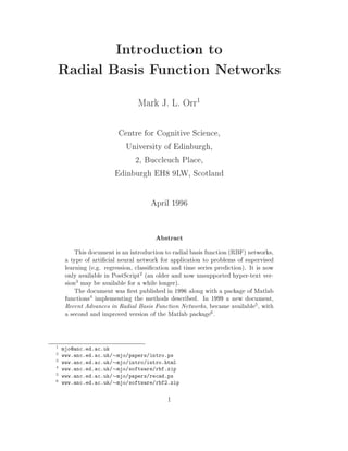
21. UEV, FPE, GCV and BIC are all in the form ^XYZ = ;XYZ y>P2 y=p and have
2
^ ^
a natural ordering,
;UEV ;FPE ;GCV ;BIC
as is plain if the ; factors are expanded out in Taylor series.
p 2 3
p ; = ;UEV = 1 + p + p + p +
p+ = ; = 1+ 2 + 2 2 + 2 3 +
p; FPE
p p2 p3
p2 = ;GCV = 1 + 2p + 3p2 + 4p3 +
2 3
(p ; )2
p + (ln(p) ; 1) = ; = 1 + ln(p) + 2 + 3 +
p; BIC
p p2 p3
5.3 Example
fit (λ = 1)
target
2 data
y
0
−4 −2 0 2 4
x
Figure 7: Training set, target function and t for the example.
Figure 7 shows a set of p = 50 training input-output points sampled from the
function
y(x) = (1 + x ; 2 x2) e;x2
21

22. with added Gaussian noise of standard deviation = 0:2. We shall t this data with
an RBF network (section 3.2) with m = 50 Gaussian centres (section 3.1) coincident
with the input points in the training set and of width r = 0:5. To avoid over t we
shall use standard ridge regression (section 6.1) controlled by a single regularisation
parameter . The error predictions, as a function of , made by the various model
selection criteria are shown in gure 8. Also shown is the mean-squared-error (MSE)
between the t and the target over an independent test set.
3
10
MSE
10
2 LOO
UEV
FPE
1 GCV
10 BIC
0
10
−1
10
−2
10 −10 −5 0 5
10 10 10 10
λ
Figure 8: The various model selection criteria, plus mean-squared-error over a test
set, as a function of the regularisation parameter.
A feature of the gure is that all the criteria have a minimum which is close to
the minimum MSE, near = 1. This is why the model selection criteria are useful.
When we do not have access to the true MSE, as in any practical problem, they are
often able to select the best model (in this example, the best ) by picking out the
one with the lowest predicted error.
Two words of warning: they don't always work as e ectively as in this example
and UEV is inferior to GCV as a selection criteria 20] (and probably to the others
as well).
22

23. 6 Ridge Regression
Around the middle of the 20th century the Russian theoretician Andre Tikhonov
was working on the solution of ill-posed problems. These are mathematical prob-
lems for which no unique solution exists because, in e ect, there is not enough
information speci ed in the problem. It is necessary to supply extra information (or
assumptions) and the mathematical technique Tikhonov developed for this is known
as regularisation.
Tikhonov's work only became widely known in the West after the publication
in 1977 of his book 29]. Meanwhile, two American statisticians, Arthur Hoerl and
Robert Kennard, published a paper in 1970 11] on ridge regression, a method for
solving badly conditioned linear regression problems. Bad conditioning means nu-
merical di culties in performing the matrix inverse necessary to obtain the variance
matrix (equation 4.4). It is also a symptom of an ill-posed regression problem in
Tikhonov's sense and Hoerl & Kennard's method was in fact a crude form of regu-
larisation, known now as zero-order regularisation 25].
In the 1980's, when neural networks became popular, weight decay was one of
a number of techniques `invented' to help prune unimportant network connections.
However, it was soon recognised 8] that weight decay involves adding the same
penalty term to the sum-squared-error as in ridge regression. Weight-decay and
ridge regression are equivalent.
While it is admittedly crude, I like ridge regression because it is mathematically
and computationally convenient and consequently other forms of regularisation are
rather ignored here. If the reader is interested in higher-order regularisation I suggest
looking at 25] for a general overview and 16] for a speci c example (second-order
regularisation in RBF networks).
We next describe ridge regression from the perspective of bias and variance
(section 6.1) and how it a ects the equations for the optimal weight vector (appendix
A.4), the variance matrix (appendix A.5) and the projection matrix (appendix A.6).
A method to select a good value for the regularisation parameter, based on a re-
estimation formula (section 6.2), is then presented. Next comes a generalisation
of ridge regression which, if radial basis functions (section 3.1) are used, can be
justly called local ridge regression (section 6.3). It involves multiple regularisation
parameters and we describe a method (section 6.4) for their optimisation. Finally,
we illustrate with a simple example (section 6.5).
6.1 Bias and Variance
When the input is x the trained model predicts the output as f (x). If we had many
training sets (which we never do but just suppose) and if we knew the true output,
y(x), we could calculate the mean-squared-error as
MSE = (y(x) ; f (x))2
23

24. where the expectation (averaging) indicated by h: : :i is taken over the training sets.
This score, which tells us how good the average prediction is, can be broken down
into two components 5], namely
MSE = (y(x) ; hf (x)i)2 + (f (x) ; hf (x)i)2 :
The rst part is the bias and the second part is the variance.
If hf (x)i = y(x) for all x then the model is unbiased (the bias is zero). However,
an unbiased model may still have a large mean-squared-error if it has a large variance.
This will be the case if f (x) is highly sensitive to the peculiarities (such as noise and
the choice of sample points) of each particular training set and it is this sensitivity
which causes regression problems to be ill-posed in the Tikhonov 29] sense. Often,
however, the variance can be signi cantly reduced by deliberately introducing a
small amount of bias so that the net e ect is a reduction in mean-squared-error.
Introducing bias is equivalent to restricting the range of functions for which a
model can account. Typically this is achieved by removing degrees of freedom.
Examples would be lowering the order of a polynomial or reducing the number of
weights in a neural network. Ridge regression does not explicitly remove degrees of
freedom but instead reduces the e ective number of parameters (section 4.4). The
resulting loss of exibility makes the model less sensitive.
A convenient, if somewhat arbitrary, method of restricting the exibility of linear
models (section 3) is to augment the sum-squared-error (equation 4.1) with a term
which penalises large weights,
p
X m
X
C = (^i ; f (xi)) +
y 2
wj2 : (6.1)
i=1 j =1
This is ridge regression (weight decay) and the regularisation parameter > 0
controls the balance between tting the data and avoiding the penalty. A small
value for means the data can be t tightly without causing a large penalty a large
value for means a tight t has to be sacri ced if it requires large weights. The bias
introduced favours solutions involving small weights and the e ect is to smooth the
output function since large weights are usually required to produce a highly variable
(rough) output function.
The optimal weight vector for the above cost function (equation 6.1) has already
been dealt with (appendix A.4), as have the variance matrix (appendix A.5) and
the projection matrix (appendix A.6). In summary,
A = H>H + Im (6.2)
w = A;1H>y
^ ^ (6.3)
P = Ip ; H A;1H> : (6.4)
24

25. 6.2 Optimising the Regularisation Parameter
Some sort of model selection (section 5) must be used to choose a value for the
regularisation parameter . The value chosen is the one associated with the lowest
prediction error. But which method should be used to predict the error and how is
the optimal value found?
The answer to the rst question is that nobody knows for sure. The popular
choices are leave-one-out cross-validation, generalised cross-validation, nal predic-
tion error and Bayesian information criterion. Then there are also bootstrap meth-
ods 14]. Our approach will be to use the most convenient method, as long as there
are no serious objections to it, and the most convenient method is generalised cross
validation (GCV) 6]. It leads to the simplest optimisation formulae, especially in
local optimisation (section 6.4).
Since all the model selection criteria depend nonlinearly on we need a method
of nonlinear optimisation. We could use any of the standard techniques for this,
such as the Newton method, and in fact that has been done 7]. Alternatively 20],
we can exploit the fact that when the derivative of the GCV error prediction is set
to zero, the resulting equation can be manipulated so that only ^ appears on the
left hand side (see appendix A.10),
^ =
y>P2 y trace A;1 ; ^ A;2
^ ^
w>A;1 w trace (P) :
^ ^ (6.5)
This is not a solution, it is a re-estimation formula because the right hand side
depends on ^ (explicitly as well as implicitly through A;1 and P). To use it, an
initial value of ^ is chosen and used to calculate a value for the right hand side. This
leads to a new estimate and the process can be repeated until convergence.
6.3 Local Ridge Regression
Pm 2
Instead of treating all weights equally with the penalty term j =1 wj we can
treat them all separately and have a regularisation parameter associated with each
P
basis function by using m j wj2. The new cost function is
j =1
p
X m
X
C = (^i ; f (xi)) +
y 2
j wj
2
(6.6)
i=1 j =1
and is identical to the the standard form (equation 6.1) if the regularisation param-
eters are all equal ( j = ). Then the variance matrix (appendix A.5) is
;
A;1 = H>H + ;1 (6.7)
25

26. where is a diagonal matrix with the regularisation parameters, f gm , along its
j =1
diagonal. As usual, the optimal weight vector is
w = A;1H>y :
^ ^ (6.8)
and the projection matrix is
P = Ip ; H A;1H> : (6.9)
These formulae are identical to standard ridge regression (section 6.1) except for
the variance matrix where Im has been replaced by .
In general there is nothing local about this form of weight decay. However, if we
con ne ourselves to local basis functions such as radial functions (section 3.1) (but
not the multiquadric type which are seldom used in practice) then the smoothness
produced by this form of ridge regression is controlled in a local fashion by the
individual regularisation parameters. That is why we call it local ridge regression
and it provides a mechanism to adapt smoothness to local conditions. Standard
ridge regression, with just one parameter, , to control the bias/variance trade-o ,
has di culty with functions which have signi cantly di erent smoothness in di erent
parts of the input space.
6.4 Optimising the Regularisation Parameters
To take advantage of the adaptive smoothing capability provided by local ridge
regression requires the use of model selection criteria (section 5) to optimise the
regularisation parameters. Information about how much smoothing to apply in
di erent parts of the input space may be present in the data and the model selection
criteria can help to extract it.
The selection criteria depend mainly on the projection matrix (equation 6.9) P
and therefore we need to deduce its dependence on the individual regularisation
parameters. The relevant relationship (equation A.6) is one of the incremental
operations (section 4.3). Adapting the notation somewhat, it is
P = Pj ; P+hh>PPh
j j h> j
j
(6.10)
j j j j
where Pj is the projection matrix after the j -th basis function has been removed
and hj is the j -th column of the design matrix (equation 4.3).
In contrast to the case of standard ridge regression (section 6.2), there is an
analytic solution for the optimal value of j based on GCV minimisation 19] {
no re-estimation is necessary (see appendix A.11). The trouble is that there are
m ; 1 other parameters to optimise and each time one j is optimised it changes
26

27. the optimal value of each of the others. Optimising all the parameters together has
to be done as a kind of re-estimation, doing one at a time and then repeating until
they all converge 19].
When j = 1 the two projection matrices, P and Pj are equal. This means
that if the optimal value of j is 1 then the j -th basis function can be removed
from the network. In practice, especially if the network is initially very exible (high
variance, low bias { see section 6.1) in nite optimal values are very common and
local ridge regression can be used as a method of pruning unnecessary hidden units.
The algorithm can get stuck in local minima, like any other nonlinear optimi-
sation, depending on the initial settings. For this reason it is best in practice to
give the algorithm a head start by using the results from other methods rather than
starting with random parameters. For example, standard ridge regression (section
6.1) can be used to nd the best global parameter, ^, and the local algorithm can
then start from
^j = ^ 1 j m :
Alternatively, forward selection (section 7) can be used to choose a subset, S , of the
original m basis functions in which case the local algorithm can start from
^j = 0 if j 2 S :
1 otherwise
6.5 Example
Figure 9 shows four di erent ts (the red curves) to a training set of p = 50 patterns
randomly sampled from the the sine wave
y = sin(12 x)
between x = 0 and x = 1 with Gaussian noise of standard deviation = 0:1 added.
The training set input-output pairs are shown by blue circles and the true target by
dashed magenta curves. The model used is a radial basis function network (section
3.2) with m = 50 Gaussian functions of width r = 0:05 whose positions coincide
with the training set input points. Each t uses standard ridge regression (section
6.1) but with four di erent values of the regularisation parameter .
The rst t (top left) is for = 1 10;10 and is too rough { high weights have
not been penalised enough. The last t (bottom right) is for = 1 105 and is too
smooth { high weights have been penalised too much. The other two ts are for
= 1 10;5 (top right) and = 1 (bottom left) which are just about right, there
is not much to choose between them.
27

28. λ = 0.0000000001 λ = 0.00001
1 1
0 0
y
−1 −1
0 1 0 1
λ=1 λ = 100000
1 1
0 0
y
−1 −1
0 1 0 1
x x
Figure 9: Four di erent RBF ts (solid red curves) to data (blue crosses) sampled
from a sine wave (dashed magenta curve).
(a) (b)
1
40 10
30
RMSE
0
20 10
γ
10
−1
0 −10 −5 0 5
10 −10 −5 0 5
10 10 10 10 10 10 10 10
λ λ
Figure 10: (a) and (b) RMSE as functions of . The optimal value is shown with
a star.
28

29. The variation of the e ective number of parameters (section 4.10), , as a func-
tion of is shown in gure 10(a). Clearly decreases monotonically as increases
and the RBF network loses exibility. Figure 10(b) shows root-mean-squared-error
(RMSE) as a function of . RMSE was calculated using an array of 250 noiseless
samples of the target between x = 0 and x = 1. The gure suggests 0:1 as the
best value (minimum RMSE) for the regularisation parameter.
In real applications where the target is, of course, unknown we do not, unfortu-
nately, have access to RMSE. Then we must use one of the model selection criteria
(section 5) to nd parameters like . The solid red in gure 11 shows the variation
of GCV over a range of values. The re-estimation formula (equation 6.5) based
on GCV gives ^ = 0:10 starting from the initial value of ^ = 0:01. Note, how-
ever, that had we started the re-estimation at ^ = 10;5 then the local minima, at
^ = 2:1 10;4, would have been the nal resting place. The values of and RMSE
at the optimum, ^ = 0:1, are marked with stars in gure 10.
0
10
GCV
−1
10
−2
10 −10 −5 0 5
10 10 10 10
λ
Figure 11: GCV as functions of with the optimal value shown with a star.
The values ^j = 0:1 were used to initialise a local ridge regression algorithm
which continually sweeps through the regularisation parameters optimising each in
turn until the GCV error prediction converges. This algorithm reduced the error
prediction from an initial value of ^ 2 = 0:016 at the optimal global parameter value
to ^2 = 0:009. At the same time 18 regularisation parameters ended up with an
optimal value of 1 enabling the 18 corresponding hidden units to be pruned from
the network.
29

30. 7 Forward Selection
We previously looked at ridge regression (section 6) as a means of controlling the
balance between bias and variance (section 6.1) by varying the e ective number of
parameters (section 4.4) in a linear model (section 3) of xed size.
An alternative strategy is to compare models made up of di erent subsets of
basis functions drawn from the same xed set of candidates. This is called subset
selection in statistics 26]. To nd the best subset is usually intractable | there
are 2M ; 1 subsets in a set of size M | so heuristics must be used to search a
small but hopefully interesting fraction of the space of all subsets. One of these
heuristics is called forward selection which starts with an empty subset to which is
added one basis function at a time | the one which most reduces the sum-squared-
error (equation 4.1) | until some chosen criterion, such as GCV (section 5.2), stops
decreasing. Another is backward elimination which starts with the full subset from
which is removed one basis function at a time | the one which least increases the
sum-squared-error | until, once again, the chosen criterion stops decreasing.
It is interesting to compare subset selection with the standard way of optimis-
ing neural networks. The latter involves the optimisation, by gradient descent, of
a nonlinear sum-squared-error surface in a high-dimensional space de ned by the
network parameters 8]. In RBF networks (section 3.1) the network parameters are
the centres, sizes and hidden-to-output weights. In subset selection the optimisation
algorithm searches in a discrete space of subsets of a set of hidden units with xed
centres and sizes and tries to nd the subset with the lowest prediction error (section
5). The hidden-to-output weights are not selected, they are slaved to the centres
and sizes of the chosen subset. Forward selection is also, of course, a nonlinear type
of algorithm but it has the following advantages:
There is no need to x the number of hidden units in advance.
The model selection criteria are tractable.
The computational requirements are relatively low.
In forward selection each step involves growing the network by one basis function.
Adding a new basis function is one of the incremental operations (section 4.3). The
key equation (A.5) is
Pm+1 = Pm ; Pm>fPfJ fPm
f
J >
(7.1)
J m J
which expresses the relationship between Pm, the projection matrix (equation 4.6)
for the m hidden units in the current subset, and Pm+1 , the succeeding projection
matrix if the J -th member of the full set is added. The vectors ffJ gM=1 are the
J
30

31. columns of the design matrix (equation 4.3) for the entire set of candidate basis
functions,
F = f1 f2 : : : fM ]
of which there are M (where M m).
If the J -th basis function is chosen then fJ is appended to the last column of
Hm, the design matrix of the current subset. This column is renamed hm+1 and the
new design matrix is Hm+1. The choice of basis function can be based on nding
the greatest decrease in sum-squared-error (equation 4.1). From the update rule
(equation 7.1) for the projection matrix and equation 4.8 for sum-squared-error
Sm ; Sm+1 = (y >Pm ffJ ) :
^> 2
^ ^ (7.2)
fJ Pm J
(see appendix A.12). The maximum (over 1 J M ) of this di erence is used to
nd the best basis function to add to the current network.
To decide when to stop adding further basis functions one of the model selection
criteria (section 5), such as GCV (equation 5.2), is monitored. Although the training
^
error, S , will never increase as extra functions are added, GCV will eventually stop
decreasing and start to increase as over t (section 6.1) sets in. That is the point at
which to cease adding to the network. See section 7.4 for an illustration.
7.1 Orthogonal Least Squares
Forward selection is a relatively fast algorithm but it can be speeded up even fur-
ther using a technique called orthogonal least squares 4]. This is a Gram-Schmidt
orthogonalisation process 12] which ensures that each new column added to the
design matrix of the growing subset is orthogonal to all previous columns. This
simpli es the equation for the change in sum-squared-error and results in a more
e cient algorithm.
Any matrix can be factored into the product of a matrix with orthogonal columns
and a matrix which is upper triangular. In particular, the design matrix (equation
4.3), Hm 2 Rp m, can be factored into
~
Hm = Hm Um (7.3)
where
~ ~ ~ ~
Hm = h1 h2 : : : hm ] 2 Rp m
~i ~
has orthogonal columns (h>hj = 0 i 6= j ) and Um 2 Rm m is upper triangular.
31

32. When considering whether to add the basis function corresponding to the J -
th column, fJ , of the full design matrix the projection of fJ in the space already
spanned by the m columns of the current design matrix is irrelevant. Only its
projection perpendicular to this space, namely
m >~
~J = fJ ; X fJ>hj hj
f ~
j =1
~ ~hj hj
can contribute to a further reduction in the training error, and this reduction is
^ ^ ^>~ 2
Sm ; Sm+1 = (y >f~J ) (7.4)
~J fJ
f
as shown in appendix A.13. Computing this change in sum-squared-error requires
of order p oating point operations, compared with p2 for the unnormalised ver-
sion (equation 7.2). This is the basis of the increased e ciency of orthogonal least
squares.
A small overhead is necessary to maintain the columns of the full design matrix
orthogonal to the space spanned by the columns of the growing design matrix and
to update the upper triangular matrix. After ~J is selected the new orthogonalised
f
full design matrix is
~ ~ ~J ~
Fm+1 = Fm ; fJ~f>~Fm
>
~
fJ fJ
and the upper triangular matrix is updated to
~m ~ ~m
Um;1 (H> ;1Hm;1);1 H> ;1fJ :
Um = 0m;1
> 1
~
Initially U1 = 1 and F0 = F. The orthogonalised optimal weight vector,
;1 >
~m~
wm = H> Hm
~ H y^ m
and the unorthogonalised optimal weight (equation 4.5) are then related by
wm = U;1 wm
^ m ~
(see appendix A.13).
7.2 Regularised Forward Selection
Forward selection and standard ridge regression (section 6.1) can be combined, lead-
ing to a modest improvement in performance 20]. In this case the key equation (7.5)
involves the regularisation parameter .
32

33. Pm+1 = Pm ; P+ ffJ>fP Pfm
m J >
(7.5)
J m J
The search for the maximum decrease in the sum-squared-error (equation 4.1) is
then based on
Sm ; Sm+1 = 2 y Pmff>P Pm fJ ; (y( P+ fJ )PfJ fP)m fJ
^ ^ ^ > 2 J y>
^
+ J m fJ
^> m f 2 > 2
> 2
(7.6)
J m J
(see appendix A.14). Alternatively, it is possible to search for the maximum decrease
in the cost function (equation 6.1)
Cm ; Cm+1 = (y f >m fJ )f :
^ ^ ^>P 2
+ J Pm J
(7.7)
(see appendix A.14).
The advantage of ridge regression is that the regularisation parameter can be
optimised (section 6.2) in between the addition of new basis functions. Since new
additions will cause a change in the optimal value anyway, there is little point in
running the re-estimation formula (equation 6.5) to convergence. Good practical
results have been obtained by performing only a single iteration of the re-estimation
formula after each new selection 20].
7.3 Regularised Orthogonal Least Squares
Orthogonal least squares (section7.1) works because after factoring Hm the orthog-
onalised variance matrix (equation 4.4) is diagonal.
;
A;1 = H> Hm ;1
m m
;1 ; > ;1
m ~m~
= U;1 H> Hm U m
2 3
1
h> h1
~1 ~ 0 ::: 0
6 0 h>1h2 ::: 0 7;
;1 6
= Um 6 ~2 ~ 7 > ;1
7 Um
6
4
... ... ... ... 7
5
0 0 ::: 1
h> h m
~m ~
;
m ~
= U;1 A;1 U> ;1 :
m
33

34. ~
A;1 is simple to compute while the inverse of the upper triangular matrix is not
required to calculate the change in sum-squared-error. However, when standard
ridge regression (section 6.1) is used
;
A;1 = H> Hm + Im ;1
m m
;1
m ~m~
= U> H> Hm Um + Im
and this expression can not be simpli ed any further. A solution to this problem is
to slightly alter the nature of the regularisation so that
;
A;1 = H> Hm + U> Um ;1
m m m
;1 ; >
~m~
= U;1 H> Hm + Im
m Um ;1
2 3
1
+h> h1
~1 ~ 0 ::: 0
6
6 0 1
::: 0 7;
7 > ;1
+h> h2
= U;1 6
m 6 ...
~2 ~
... ... ... 7 Um
7
4 5
0 0 ::: 1
+h> hm
~m ~
;
m ~
= U;1 A;1 U> ;1 :
m
This means that instead of the normal cost function (equation 6.1) for standard
ridge regression (section 6.1) the cost is actually
Cm = (y ; Hm w)>(y ; Hm w) + wmU> Um wm :
^ ^ >
m (7.8)
Then the change in sum-squared-error is
~>~ ) ^>~ 2
Sm ; Sm+1 = (2 + fJ f~J>~(y2 fJ ) :
^ ^ (7.9)
( + fJ fJ )
Alternatively, searching for the best basis function to add could be made on the
basis of the change in cost, which is simply
^ ^ ^>~ 2
Cm ; Cm+1 = (y ~J )~ :
f (7.10)
+ fJ fJ
>
For details see appendix A.15.
34

35. 7.4 Example
Figure 12 shows a set of p = 50 training examples sampled with Gaussian noise of
standard deviation = 0:1 from the logistic function
y(x) = 1 ; e;x :
1+
e;x
fit
1 target
data
y
0
−1
−10 −5 0 5 10
x
Figure 12: Training set, target function and forward selection t.
This data is to be modeled by forward selection from a set of M = 50 Gaussian
radial functions (section 3.1) coincident with the training set inputs and of width
r = 2. Figure 13 shows the sum-squared-error (equation 4.1), generalised cross-
validation (equation 5.2) and the mean-squared-error between the t and target
(based on an independent test set) as new basis functions are added one at a time.
The training set error monotonically decreases as more basis functions are added
but the GCV error prediction eventually starts to increase (at the point marked
with a star). This is the signal to stop adding basis functions (which in this example
occurs after the RBF network has acquired 13 basis functions) and happily coincides
with the minimum test set error. The t with these 13 basis functions is shown in
gure 12. Further additions only serve to make GCV and MSE worse. Eventually,
after about 19 additions, the variance matrix (equation 4.4) becomes ill-conditioned
when numerical calculations are unreliable.
35

36. 0
10
MSE
GCV
SSE
−1
10
−2
10 ill−conditioned
−3
10
0 10 20 30 40 50
iteration number
Figure 13: The progress of SSE, GCV and MSE as new basis functions are added in
plain vanilla forward selection. The minimum GCV, and corresponding MSE, are
marked with stars. After about 19 selections the variance matrix becomes badly
conditioned.
0
10
MSE
GCV
SSE
−1
10
−2
10
−3
10
0 10 20 30 40 50
iteration number
Figure 14: The progress of SSE, GCV and MSE as new basis functions are added
in regularised forward selection.
36

37. The results of using regularised forward selection (section 7.2) are shown in gure
14. The sum-squared-error (equation 4.1) no longer decreases monotonically because
^ is re-estimated after each selection. Also, regularisation prevents the variance
matrix (equation 4.4) becoming ill-conditioned, even after all the candidate basis
functions are in the subset.
In this example the two methods chose similar (but not identical) subsets and
ended with very close test set errors. However, on average, over a large number of
similar training sets, the regularised version performs slightly better than the plain
vanilla version 20].
37

38. A Appendices
A.1 Notational Conventions
Scalars are represented by italicised letters such as y or . Vectors are represented
by bold lower case letters such as x and . The rst component of x (a vector)
is x1 (a scalar). Vectors are single-column matrices, so, for example, if x has n
components then
2 3
x1
6 x2 7
x = 6 .. 7 :
6 7
4 . 5
xn
Matrices, such as H, are represented by bold capital letters. If the rows of H are
indexed by i and the columns by j then the entry in the i-th row and j -th column
of H is Hij . If H has p rows and m columns (H 2 Rp m ) then
2 3
H11 H12 : : : H1m
6 H H ::: H 7
H = 6 ..21 ..22 . . . ..2m 7 :
6
4 . 7
. . 5
Hp1 Hp2 : : : Hpm
The transpose of a matrix { the rows and columns swapped { is represented by
H>. So, for example, if G = H> then
Gji = Hij :
The transpose of a vector is a single-row matrix: x> = x1 x2 : : : xn]. It follows
that x = x1 x2 : : : xn]> which is a useful way of writing vectors on a single line.
Also, the common operation of vector dot-product can be written as the transpose
of one vector multiplied by the other vector. So instead of writing x y we can just
write x>y.
The identity matrix, written I, is a square matrix (one with equal numbers of
rows and columns) with diagonal entries of 1 and zero elsewhere. The dimension is
written as a subscript, as in Im, which is the identity matrix of size m (m rows and
m columns).
The inverse of a square matrix A is written A;1. If A has m rows and m columns
then
A;1 A = A A;1 = Im
which de nes the inverse operation.
Estimated or uncertain values are distinguished by the use of the hat symbol.
For example, ^ is an estimated value for , and w is an estimate of w.
^
38

39. A.2 Useful Properties of Matrices
Some useful de nitions and properties of matrices are given below and illustrated
with some of the matrices (and vectors) commonly appearing in the main text.
The elements of a diagonal matrix are zero o the diagonal. An example is the
matrix of regularisation parameters appearing in equation 6.8 for the optimal weight
in local ridge regression
2 3
1 0 ::: 0
6 0 2 ::: 0 7
= 6 .. .. . . .. 7 :
6
4 . . . . 7 5
0 0 ::: m
Non-square matrices can also be diagonal. If M is any matrix then it is diagonal if
Mij = 0 i 6= j .
A symmetric matrix is identical to its own transpose. Example are the vari-
ance matrix (equation 4.4) A;1 2 Rm m and the projection matrix (equation 4.6)
P 2 Rp p. Any square diagonal matrix, such as the identity matrix, is necessarily
symmetric.
The inverse of an orthogonal matrix is its own transpose. If V is orthogonal then
V>V = V V> = Im :
Any matrix can be decomposed into the product of two orthogonal matrices and a
diagonal one. This is called singular value decomposition (SVD) 12]. For example,
the design matrix (equation 4.3) H 2 Rp m decomposes into
H = U V>
where U 2 Rp p and V 2 Rm m are orthogonal and 2 Rp m is diagonal.
The trace of a square matrix is the sum of its diagonal elements. The trace of
the product of a sequence of matrices is una ected by rotation of the order. For
example,
; ;
trace H A;1 H> = trace A;1 H>H :
The transpose of a product is equal to the product of the individual transposes
in reverse order. For example,
; ;1 > >
A H y = y>H A;1 :
^ ^
A;1 is symmetric so (A;1)> = A;1.
The inverse of a product of square matrices is equal to the product of the indi-
vidual inverses in reverse order. For example,
; > > ;1 ;
V V = V > ;1 V > :
V is orthogonal so V;1 = V> and (V>);1 = V.
39

40. A.3 Radial Basis Functions
The most general formula for any radial basis function (RBF) is
;
h(x) = (x ; c)>R;1(x ; c)
where is the function used (Gaussian, multiquadric, etc...), c is the centre and R is
the metric. The term (x ; c)>R;1(x ; c) is the distance between the input x and the
centre c in the metric de ned by R. There are several common types of functions
used, for example, the Gaussian, (z)1= e;z , the multiquadric, (z) = (1 + z) 1 , the
2
inverse multiquadric, (z) = (1 + z) ; 2 and the Cauchy (z ) = (1 + z );1 .
Often the metric is Euclidean. In this case R = r2 I for some scalar radius r and
the above equation simpli es to
h(x) = (x ; c)>(x ; c) :
r2
A further simpli cation is a 1-dimensional input space in which case we have
h(x) = (x ; c)2 :
r2
This function is illustrated for c = 0 and r = 1 in gure 15 for the above RBF types.
2
1
0
−2 0 2
Figure 15: Gaussian (green), multiquadric (magenta), inverse-multiquadric (red)
and Cauchy (cyan) RBFs all of unit radius and all centred at the origin.
40

41. A.4 The Optimal Weight Vector
As is well known from elementary calculus, to nd an extremum of a function you
1. di erentiate the function with respect to the free variable(s),
2. equate the result(s) with zero, and
3. solve the resulting equation(s).
In the case of least squares (section 4) applied to supervised learning (section 2)
with a linear model (section 3) the function to be minimised is the sum-squared-error
Xp
S = (^i ; f (xi))2
y
i=1
where
m
X
f (x) = wj hj (x)
j =1
and the free variables are the weights fwj gm .
j =1
To avoid repeating two very similar analyses we shall nd the minimum not of
S but of the cost function
Xp m
X
C = (^i ; f (xi)) +
y 2
j wj
2
i=1 j =1
used in ridge regression (section 6). This includes an additional weight penalty term
controlled by the values of the non-negative regularisation parameters, f gm . To
j =1
get back to ordinary least squares (without any weight penalty) is simply a matter
of setting all the regularisation parameters to zero.
So, let us carry out this optimisation for the j -th weight. First, di erentiating
the cost function
p
@C = 2 X (f (x ) ; y ) @f (x ) + 2 w :
^i @w i
i j j
@wj i=1 j
We now need the derivative of the model which, because the model is linear, is
particularly simple.
@f (x ) = h (x ) :
@wj i j i
Substituting this into the derivative of the cost function and equating the result to
zero leads to the equation
Xp Xp
f (xi) hj (xi) + j wj =
^ yi hj (xi ) :
^
i=1 i=1
41

42. There are m such equations, for 1 j m, each representing one constraint on
the solution. Since there are exactly as many constraints as there are unknowns
the system of equations has, except under certain pathological conditions, a unique
solution.
To nd that unique solution we employ the language of matrices and vectors:
linear algebra. These are invaluable for the representation and analysis of systems
of linear equations like the one above which can be rewritten in vector notation (see
appendix A.1) as follows.
h>f + j wj = h>y
j ^ j^
where
2 3 2 3 2 3
hj (x1 ) f (x1 ) y1
^
6 hj (x2 ) 7 6 f (x2 ) 7 6 y2 7
^
hj = 6 .. 7 f = 6 .. 7 y = 6 .. 7 :
6
4 . 5 7 6
4 . 5 7 ^ 6 74 . 5
hj (xp) f (xp) yp
^
Since there is one of these equations (each relating one scalar quantity to another)
for each value of j from 1 up to m we can stack them, one on top of another, to
create a relation between two vector quantities.
2 > 3 2 3 2 > 3
h1 f 1 w1
^ hy ^
6 h>f 7 6 2 w2 7
6 2 7+6 ^ 6 h1 y 7
>^
6 . 7 6 . 7 = 6 2. 7 :
4 . 5 4 . 7 6 . 7
. . 5 4 . 5
hm>f m wm
^ h> y
m^
However, using the laws of matrix multiplication, this is just equivalent to
H>f + w = H>y
^ ^ (A.1)
where
2 3
1 0 ::: 0
6 0 2 ::: 0 7
= 6
6 7
... ... . . . ... 7 :
4 5
0 0 ::: m
and where H, which is called the design matrix, has the vectors fhj gm as its
j =1
columns,
H = h1 h2 : : : hm ]
and has p rows, one for each pattern in the training set. Written out in full it is
2 3
h1(x1 ) h2 (x1) : : : hm (x1)
6 h (x ) h (x ) : : : h (x ) 7
H = 6 1 .. 2 2 .. 2 . . . m .. 2 7
6
4 . 7
. . 5
h1(xp) h2 (xp) : : : hm(xp)
42