Chapter2 gis fundamentals

23
2 Data Models
Introduction
Data in a GIS represent a simplified view
of the real world. Physical entities or phe-
nomena are approximated by data in a GIS.
These data include information on the spatial
location and extent of the physical entities,
and information on their non-spatial proper-
ties.
Each entity is represented by a spatial
feature or cartogaphic object in the GIS, and
so there is an entity-object correspondence.
Because every computer system has limits,
only a subset of the essential characteristics
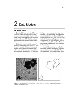
are represented for each entity. As illustrated
in Figure 2-1, we may represent lakes in a
region by a set of polygons. These polygons
are associated with a set of essential charac-
teristics that define each lake. All other infor-
mation for the area may be ignored, e.g.,
information on the roads, buildings, slope, or
soil characteristics. Only lake boundaries and
essential lake characteristics have been saved
in this example.
Essential characteristics are defined by
the person, group, or organization that devel-
ops the spatial data or uses the GIS. The set
of characteristics used to represent an entity
Figure 2-1: A physical entity is represented by a spatial object in a GIS. Here, the physical boundaries of
lakes are represented by lines.

24 GIS Fundamentals
is subjectively chosen. What is essential to
describe a forest for one person, for example
a logger, would be different than what is
essential to another person, such as a typical
member of the Sierra Club. Objects are
abstractions in a spatial database, because
we can only record and maintain a subset of
characteristics of any entity, and no one
abstraction is universally better than any
other.
A data model may be defined as the
objects in a spatial database plus the rela-
tionships among them. The term model is
fraught with ambiguity, because it is used in
many disciplines to describe many things.
Here the purpose of a spatial data model is to
provide a formal means of representing and
manipulating spatially-referenced informa-
tion. In our lake example our data model
consists of two parts. The first part is a set of
polygons (closed areas) recording the shore-
line of the lake, and the second part is a set
of numbers or letters associated with each
polygon. A data model may be considered
the most recognizable level in our computer
abstraction of the real world. Data structures
and binary machine code are successively
less recognizable, but more computer-com-
patible forms of the spatial data (Figure 2-2).
Coordinates are used to define the spa-
tial location and extent of geographic
objects. A coordinate most often consists of
a pair of numbers that specify location in
relation to an origin. The coordinates quan-
Figure 2-2: Levels of abstraction in the representation of spatial entities. The real world is repre-
sented in successively more machine-compatible but humanly obscure forms.

Chapter 2: Data Models 25
tify the distance from the origin when mea-
sured along a standard direction. Single or
groups of coordinates are organized to repre-
sent the shapes and boundaries that define
the objects. Coordinate information is an
important part of the data model, and models
differ in how they represent these coordi-
nates. Coordinates are usually expressed in
one of many standard coordinate systems.
The coordinate systems are usually based
upon standardized map projections (dis-
cussed in Chapter 3) that unambiguously
define the coordinate values for every point
in an area.
Typically there are two distinct types of
data used to define cartographic objects
(Figure 2-3). First, coordinate or geometric
data define the location and shape of the
objects. Second, attribute data are collected
and referenced to each object. These
attribute data record the non-spatial compo-
nents of an object, such as a name, color, pH,
or cash value.
Attribute data are linked with coordinate
data to help define each cartographic object
in the GIS. The attribute data are linked to
the corresponding cartographic objects in the
spatial part of the GIS database. Keys,
labels, or other indices are used so that the
spatial and attribute data may be viewed,
related, and manipulated together.
Most conceptualizations view the world
as a set of layers (Figure 2-4). Each layer
organizes the spatial and attribute data for a
given set of cartographic objects in the
region of interest. These are often referred to
as thematic layers. As an example consider a
GIS database that includes a soils data layer,
a population data layer, an elevation data
layer, and a roads data layer. The roads layer
“contains” only roads data, including the
location and properties of roads in the analy-
sis area. There are no data regarding the
location and properties of any other geo-
graphic entities in the roads layer. Informa-
tion on soils, population, and elevation are
Figure 2-3: Coordinate and attribute data are used to represent entities.

26 GIS Fundamentals
contained in their respective data layers.
Through analyses we may combine data to
create a new data layer, e.g., we may identify
areas that are “high” elevation and join this
information with the soils data. This join
creates a new data layer with a new, compos-
ite soils/elevation variable mapped.
Coordinate Data
Coordinates define location in two or
three-dimensional space. Coordinate pairs,
e.g., x and y, or coordinate triples, x, y, and z,
are used to define the shape and location of
each spatial object or phenomenon.
Spatial data in a GIS most often use a
Cartesian coordinate system, so named after
Rene Descartes, a French mathematician.
Cartesian systems define two or three
orthogonal (right-angle) axes. Two-dimen-
sional Cartesian systems define x and y axes
in a plane (Figure 2-5, left) Three-dimen-
sional Cartesian systems define a z axis,
orthogonal to both the x and y axes. An ori-
gin is defined with zero values at the inter-
Figure 2-4: Spatial data are most often viewed
as a set of thematically distinct layers.
Figure 2-5: Cartesian (left) and spherical (right) coordinate systems.

section of the orthogonal axes. Cartesian
coordinates are usually specified as decimal
numbers, by convention increasing from bot-
tom to top and from left to right.
Coordinate data may also be specified in
a spherical coordinate system. Hipparchus, a
Greek mathematician of the 2nd century
B.C., was among the first to specify loca-
tions on the Earth using angular measure-
ments on a sphere. The most common
spherical system uses two angles of rotation
and a radius distance, r, to specify locations
on a modeled earth surface (Figure 2-5,
right). These angles of rotation occur around
a polar axis to define a longitude (λ) and
with reference to an equatorial plane to
define a latitude (φ). Latitudes increase from
zero at the Equator to 90 degrees at the
poles. Northern latitudes are preceded by an
N and southern latitudes by an S, e.g., N90o
,
S10o. Longitudes increase east and west of
an origin. Longitude values are preceded by
an E and W, respectively, e.g., W110o
.
Northern and eastern directions are desig-
nated as positive and southern and western
designated as negative when signed coordi-
nates are required. Spherical coordinates are
most often recorded in a degrees-minutes-
seconds (DMS) notation, e.g. N43o
35’ 20”,
signifying 43 degrees, 35 minutes, and 20
seconds of latitude. Minutes and seconds
range from zero to sixty. Alternatively,
spherical coordinates may be expressed as
decimal degrees (DD). DMS may be con-
verted to DD by:
DD = DEG + MIN/60 + SEC/3600 (2.1)
Attribute Data and Types
Attribute data are used to record the
non-spatial characteristics of an entity.
Attributes are also called items or variables.
Attributes may be envisioned as a list of
characteristics that help describe and define
the features we wish to represent in a GIS.
Color, depth, weight, owner, component
vegetation type, or landuse are examples of
variables that may be used as attributes.
Attributes have values, e.g., color may be
blue, black or brown, weight from 0.0 to
500.0, or landuse may be urban, agriculture,
or undeveloped. Attributes are often pre-
sented in tables, with attributes arranged in
rows and columns (Figure 2-2). Each row
corresponds to an individual spatial object,
and each column corresponds to an attribute.
Tables are often organized and managed
using a specialized computer program called
a database management system (DBMS,
described fully in Chapter 8).
Attributes of different types may be
grouped together to describe the non-spatial
properties of each object in the database.
These attribute data may take many forms,
but all attributes can be categorized as nomi-
nal, ordinal, or interval/ratio attributes.
Nominal attributes are variables that
provide descriptive information about an
object. Color, a vegetation type, a city name,
the owner of a parcel, or soil series are all
examples of nominal attributes. There is no
implied order, size, or quantitative informa-
tion contained in the nominal attributes.
Nominal attributes may also be images,
film clips, audio recordings, or other
descriptive information. Just as the color or
type attributes provide nominal information
for an entity, an image may also provide
descriptive information. GIS for real estate
management and sales often have images of
the buildings or surroundings as part of the
database. Digital images provide informa-
tion not easily conveyed in any other man-
ner. These image or sound attributes are
sometimes referred to as BLOBs for binary
large objects, but they are best considered as
a special case of a nominal attribute.
Ordinal attributes imply a rank order or
scale by their values. An ordinal attribute
may be descriptive such as small, medium,
or large, or they may be numeric, such as an
erosion class which takes values from 1
through 10. The order reflects only rank, and
does not specify the form of the scale. An
object with an ordinal attribute that has a
value of four has a higher rank for that

28 GIS Fundamentals
attribute than an object with a value of two.
However we cannot infer that the attribute
value is twice as large, because we cannot
assume the scale is linear.
Interval/ratio attributes are used for
numeric items where both order and absolute
difference in magnitudes are reflected in the
numbers. These data are often recorded as
real numbers, most often on a linear scale.
Area, length, weight, value, height, or depth
are a few examples of attributes which are
represented by interval/ratio variables.
Common Spatial Data Models
Spatial data models begin with a con-
ceptualization, a view of real world phenom-
ena or entities. Consider a road map suitable
for use at a statewide or provincial level.
This map is based on a conceptualization
that defines roads as lines. These lines con-
nect cities and towns that are shown as dis-
crete points or polygons on the map. Road
properties may include only the road type,
e.g., a limited access interstate, state high-
way, county road, or some other type of
road. The roads have a width represented by
the drawing symbol on the map, however
this width, when scaled, may not represent
the true road width. This conceptualization
identifies each road as a linear feature that
fits into a small number of categories. All
state highways are represented by the same
type of line, even though the state highways
may vary. Some may be paved with con-
crete, others with bitumen. Some may have
wide shoulders, others not, or dividing barri-
ers of concrete, versus a broad vegetated
median. We realize these differences can
exist within this conceptualization.
There are two main conceptualizations
used for digital spatial data. The first con-
ceptualization defines discrete objects using
a vector data model. Vector data models use
discrete elements such as points, lines, and
polygons to represent the geometry of real-
world entities (Figure 2-6).
A farm field, a road, a wetland, cities,
and census tracts are examples of discrete
entities that may be represented by discrete
objects. Points are used to define the loca-
tions of “small” objects such as wells, build-
ings, or ponds. Lines may be used to
represent linear objects, e.g., rivers or roads,
or to identify the boundary between what is a
part of the object and what is not a part of
the object. We may map landcover for a
region of interest, and we categorize discrete
areas as a uniform landcover type. A forest
may share an edge with a pasture, and this
boundary is represented by lines. The
boundaries between two polygons may not
be discrete on the ground, for example, a for-
est edge may grade into a mix of trees and
grass, then to pasture; however in the vector
conceptualization, a line between two land-
cover types will be drawn to indicate a dis-
crete, abrupt transition between the two
types. Lines and points have coordinate loca-
tions, but points have no dimension, and
lines have no dimension perpendicular to
their direction. Area features may be defined
by a closed, connected set of lines.
The second common conceptualization
identifies and represents grid cells for a
given region of interest. This conceptualiza-
tion employs a raster data model (Figure 2-
6). Raster cells are arrayed in a row and col-
umn pattern to provide “wall-to-wall” cover-
age of a study region. Cell values are used to
represent the type or quality of mapped vari-
ables. The raster model is used most com-
monly with variables that may change
continuously across a region. Elevation,
mean temperature, slope, average rainfall,
cumulative ozone exposure, or soil moisture
are examples of phenomena that are often
represented as continuous fields. Raster rep-
resentations are commonly used to represent
discrete features, for example, class maps
such as vegetation or political units.

Data models are at times interchange-
able in that many phenomena may be repre-
sented with either the vector or raster
conceptual approach. For example, elevation
may be represented as a surface (continuous
field) or as series of lines representing con-
tours of equal elevation (discrete objects).
Data may be converted from one conceptual
view to another, e.g., the location of contour
lines (lines of equal elevation) may be deter-
mined by evaluating the raster surface, or a
raster data layer may be derived from a set of
contour lines. These conversions entail some
costs both computationally and perhaps in
data accuracy.
The selection of a raster or vector con-
ceptualization often depends on the type of
operations to be performed. For example,
slope is more easily determined when eleva-
tion is represented as a continuous field in a
raster data set. However, discrete contours
are often the preferred format for printed
maps, so the discrete conceptualization of a
vector data model may be preferred for this
application. The best data model for a given
organization or application depends on the
most common operations, the experiences
and views of the GIS users, the form of
available data, and the influence of the data
model on data quality.
In addition to the two main data models,
there are other data models that may be
described as variants, hybrids, or special
forms by some GIS users, and as different
families of data models by others. A triangu-
lated irregular network (TIN) is an example
of such a data model. This model is most
often used to represent surfaces, such as ele-
vations, through a combination of point, line,
and area features. Many consider this a spe-
cial, admittedly well-developed, type of vec-
tor data model. Variants or other
representations related to raster data models
also exist. We choose two broad categories
for clarity in an introductory text, and intro-
duce variants as appropriate later in this and
other chapters.
Figure 2-6: Vector and raster data models.

30 GIS Fundamentals
Vector data models will be described in
the next section, including commonly found
variants. Sections describing raster data
models, TIN data models, and data structure
then follow.
Vector Data Models
A vector data model uses sets of coordi-
nates and associated attribute data to define
discrete objects. Groups of coordinates
define the location and boundaries of dis-
crete objects, and these coordinate data plus
associated attributes are used to create vector
objects representing the real-world entities
(Figure 2-7).
There are three basic types of vector
objects: points, lines, and polygons (Figure
2-8). A point uses a single coordinate pair to
represent the location of an entity that is con-
sidered to have no dimension. Gas wells,
light poles, accident location, and survey
points are examples of entities often repre-
sented as point objects in a spatial database.
Some of these have real physical dimension,
but for the purposes of the GIS users they
may be represented as points. In effect, this
means the size or dimension of the entity is
not important spatial information, only the
central location. Attribute data are attached
to each point, and these attribute data record
the important non-spatial characteristics of
the point entities. When using a point to rep-
resent a light pole, important attribute infor-
mation might be the height of the pole, the
type of light and power source, and the last
date the pole was serviced.
Figure 2-7: Coordinates define spatial location and shape. Attributes record the important non-spatial
characteristics of features in a vector data model.

Linear features, often referred to as arcs,
are represented as lines when using vector
data models. Lines are most often repre-
sented as an ordered set of coordinate pairs.
Each line is made up of line segments that
run between adjacent coordinates in the
ordered set (Figure 2-8). A long, straight line
may be represented by two coordinate pairs,
one at the start and one at the end of the line.
Curved linear entities are most often repre-
sented as a collection of short, straight, line
segments, although curved lines are at times
represented by a mathematical equation
describing a geometric shape. Lines typi-
cally have a starting point, an ending point,
and intermediate points to represent the
shape of the linear entity. Starting points and
ending points for a line are sometimes
referred to as nodes, while intermediate
points in a line are referred to as vertices
(Figure 2-8). Attributes may be attached to
the whole line, line segments, or to nodes
and vertices along the lines
Area entities are most often represented
by closed polygons. These polygons are
formed by a set of connected lines, either
one line with an ending point that connects
back to the starting point, or as a set of lines
connected start-to-end (Figure 2-8). Poly-
gons have an interior region and may
entirely enclose other polygons in this
region. Polygons may be adjacent to other
polygons and thus share “bordering” or
“edge” lines with other polygons. Attribute
data may be attached to the polygons, e.g.,
area, perimeter, landcover type, or county
name may be linked to each polygon.
The Spaghetti Vector Model
The spaghetti model is an early vector
data model that was originally developed to
organize and manipulate line data. Lines are
captured individually with explicit starting
and ending nodes, and intervening vertices
used to define the shape of the line. The spa-
ghetti model records each line separately.
The model does not explicitly enforce or
record connections of line segments when
they cross, nor when two line ends meet
(Figure 2-9a). A shared polygon boundary
may be represented twice, with a line for
each polygon on either side of the boundary.
Data in this form are similar in some
Figure 2-8: Points, nodes and vertices define points, line, and polygon features
in a vector data model.

32 GIS Fundamentals
respects to a plate of cooked spaghetti, with
no ends connected and no intersections when
lines cross.
The spaghetti model is a relatively
unstructured way of representing vector
data. Because connections among lines are
not enforced there may be breaks or overlaps
in what should be a connected set of lines.
The set of lines that defines a polygon may
not form a closed area, so it is not possible to
specify the region inside vs. the region out-
side of the polygon. Coordinates for points,
lines, and polygons are often stored sequen-
tially, such that data for nearby areas may be
stored quite far apart. This significantly
slows data access.
The spaghetti model severely limits spa-
tial data analysis and is little used except
when entering spatial data. Because lines
often do not connect when they should,
many common spatial analyses are ineffi-
cient and the results incorrect. For example,
analyses such as determining an optimum set
of bus routes are precluded if all street con-
nections are not represented in a roads data
layer. Area calculation, layer overlay, and
many other analyses require “clean” spatial
data in which all polygons close and lines
meet correctly.
Topological Vector Models
Topological vector models specifically
address many of the shortcomings of spa-
ghetti data models. Early GIS developers
realized that they could greatly improve the
speed, accuracy, and utility of many spatial
data operations by enforcing strict connec-
tivity, by recording connectivity and adja-
cency, and by maintaining information on
the relationships between and among points,
lines, and polygons in spatial data. These
early developers found it useful to record
information on the topological characteris-
tics of data sets.
Topology is the study of geometric prop-
erties that do not change when the forms are
bent, stretched or undergo similar transfor-
mations. Polygon adjacency is an example of
a topologically invariant property, because
the list of neighbors to any given polygon
does not change during geometric stretching
or bending (Figure 2-9, b and c). Topological
vector models explicitly record topological
relationships such as adjacency and connec-
Figure 2-9: Spaghetti (a), topological (b), and topological-warped (c) vector data. Figures b and c are
topologically identical because they have the same connectivity and adjacency.

tivity in the data files. These relationships
may be recorded separately from the coordi-
nate data and hence do not change when data
are stretched or bent, e.g., when converting
between coordinate systems.
Topological vector models may also
enforce particular types of topological rela-
tionships. Planar topology requires that all
features occur on a two-dimensional surface.
There can be no overlaps among lines or
polygons in the same layer (Figure 2-10).
When planar topology is enforced, lines may
not cross over or under other lines. At each
line crossing there must be an intersection.
The top left of Figure 2-10 shows a non-pla-
nar graph. Four line segments coincide. At
some locations the lines intersect and a node
is present, but at some locations a line passes
over or under another line segment. These
lines are non-planar because if forced to be
in the same plane, all line crossings would
intersect at a node. The top right of Figure 2-
10 shows planar topology enforced for these
same four line segments. Nodes, shown as
white-filled circles, are found at each line
crossing.
Non-planarity may also occur for poly-
gons, as shown at the bottom of Figure 2-10.
Two polygons overlap slightly at an edge.
This may be due to an error, e.g., the two
polygons share a boundary but have been
recorded with an overlap, or there may be
two areas that overlap in some way. On the
left the polygons are non-planar, that is, they
occur one above the other. If topological pla-
narity is enforced, these two polygons must
be resolved into three separate, non-overlap-
ping polygons. Nodes are placed at the inter-
sections of the polygon boundaries (lower
right, Figure 2-10).
There are additional topological con-
structs besides planarity that may be
recorded or enforced in topological data
structures. For example, polygons may be
exhaustive, in that there are no gaps, holes or
“islands” in a set of polygons. Line direction
may be recorded, so that a “from” and “to”
node are identified in each line. Directional-
ity aids the representation of river or street
networks, where there may be a natural flow
direction.
There is no single, uniform set of topo-
logical relationships that are included in all
topological data models. Different research-
ers or software vendors have incorporated
different topological information in their
data structures. Planar topology is often
included, as are representations of adjacency
(which polygons are next to which) and con-
nectivity (which lines connect to which).
However, much of this information can be
generated “on-the-fly”, during processing.
Topological relationships may be con-
structed only as needed, each time a data
layer is accessed. Some GIS software pack-
ages create and maintain detailed topological
relationships in their data. This results in
more complex and perhaps larger data struc-
tures, but access is often faster, and topology
provides more consistent, “cleaner” data.
Other systems maintain little topological
information in the data structures, but com-
pute and act upon topology as needed during
specific processing.
Topological vector models often use
codes and tables to record topology. As
described above, nodes are the starting and
ending points of lines. Each node and line is
given a unique identifier. Sequences of
nodes and lines are recorded as a list of iden-
tifiers, and point, line, and polygon topology
recorded in a set of tables. The vector fea-
tures and tables in Figure 2-11 illustrate one
form of this topological coding.
Point topology is often quite simple.
Points are typically independent of each
other, so they may be recorded as individual
identifiers, perhaps with coordinates
included, and in no particular order (Figure
2-11, top).
Line topology typically includes sub-
stantial structure, and identifies at a mini-
mum the beginning and ending points of
each line (Figure 2-11, middle). Variables
record the topology and may be organized in
a table. These variables may include a line
identifier, the starting node, and the ending
node for each line. In addition, lines may be

34 GIS Fundamentals
assigned a direction, and the polygons to the
left and right of the lines recorded. In most
cases left and right are defined in relation to
the direction of travel from the starting node
to the ending node.
Polygon topology may also be defined
by tables (Figure 2-11, bottom). The tables
may record the polygon identifiers and the
list of connected lines that define the poly-
gon. Edge lines are often recorded in
sequential order. The lines for a polygon
form a closed loop, resulting in the starting
node of the first line in the list that also
serves as the ending node for the last line in
the list. Note that there may be a “back-
ground” polygon defined by the outside area.
This background polygon is not a closed
polygon as all the rest, however it may be
defined for consistency and to provide
entries in the line topology table.
Finally, note that there may be coordi-
nate tables (not shown in Figure 2-11) that
record the identifiers and locations of each
node, and coordinates for each vertex within
a line or polygon. Node locations are
recorded with coordinate pairs for each
node, while line locations are represented by
an identifier and a list of vertex coordinates
for each line.
Figure 2-11 illustrates the inter-related
structure inherent in the tables that record
topology. Point or node records may be
related to lines, which in turn may be related
to polygons. All these may then be linked in
complex ways to coordinate tables that
record location.
Figure 2-10: Non-planar and planar topology in lines and polygons.

Topological vector models greatly
enhance many vector data operations. Adja-
cency analyses are reduced to a table look
up, an operation that is relatively simple to
program and quick to execute in most soft-
ware systems. For example, an analyst may
want to identify all polygons adjacent to a
city. Assume the city is represented as a sin-
gle polygon. The operation reduces to 1)
scanning the polygon topology table to find
the polygon labeled city and reading the list
of lines that bound the polygon, and 2) scan-
ning this list of lines for the city polygon,
accumulating a list of all left and right poly-
gons. Polygons adjacent to the city may be
identified from this list. List searches on
topological tables are typically much faster
than searches involving coordinate data.
Topological vector models also enhance
many other spatial data operations. Network
and other connectivity analyses are con-
cerned with the flow of resources through
defined pathways. Topological vector mod-
els explicitly record the connections of a set
of pathways and so facilitate network analy-
ses. Overlay operations are also enhanced
when using topological vector models. The
mechanics of overlay operations are dis-
cussed in greater detail in Chapter 9, how-
ever we will state here that they involve
identifying line adjacency, intersection, and
resultant polygon formation. The interior
and exterior regions of existing and new
polygons must be determined, and these
regions depend on polygon topology. Hence,
Figure 2-11: An example of possible vector feature topology and tables. Additional or different
tables and data may be recorded to store topological information.

36 GIS Fundamentals
topological data are useful in many spatial
analyses.
There are limitations and disadvantages
to topological vector models. First, there are
computational costs in defining the topologi-
cal structure of a vector data layer. Software
must determine the connectivity and adja-
cency information, assign codes, and build
the topological tables. Computational costs
are typically quite modest with current com-
puter technologies.
Second, the data must be very “clean”,
in that all lines must begin and end with a
node, all lines must connect correctly, and all
polygons must be closed. Unconnected lines
or unclosed polygons will cause errors dur-
ing analyses. Significant human effort may
be required to ensure clean vector data
because each line and polygon must be
checked. Software may help by flagging or
fixing “dangling” nodes that do not connect
to other nodes, and by automatically identi-
fying all polygons. Each dangling node and
polygon may then be checked, and edited as
needed to correct errors.
These limitations are far outweighed by
the gains in efficiency and analytical capa-
bilities provided by topological vector mod-
els. Many current vector GIS packages use
topological vector models in some form.
Raster Data Models
Models and Cells
Raster data models define the world as a
regular set of cells in a grid pattern (Figure
2-12). Typically these cells are square and
evenly spaced in the x and y directions. The
phenomena or entities of interest are repre-
sented by attribute values associated with
each cell location. Raster data sets have a
cell dimension, defining the size of the cell.
The cell dimension specifies the length and
width of the cell in surface units, e.g. the cell
dimension may be specified as a square 30
meters on each side. The cells are usually
oriented parallel to the x and y directions.
Thus, if we know the cell dimension and the
coordinates of any one cell e.g., the lower
left corner, we may calculate the coordinate
of any other cell location.
Raster data models are the natural
means to represent “continuous” spatial fea-
tures or phenomena. Elevation, precipitation,
slope, and pollutant concentration are exam-
ples of continuous spatial variables. These
variables characteristically show significant
changes in value over broad areas. The gra-
dients can be quite steep (e.g., at cliffs), gen-
tle (long, sloping ridges), or quite variable
(rolling hills). Because raster data may be a
dense sampling of points in two dimensions,
they easily represent all variations in the
changing surface. Raster data models depict
these gradients by changes in the values
associated with each cell.
Square raster cells have a characteristic
cell dimension or cell size (Figure 2-12).
This cell dimension is the edge length of
each cell, and cell dimension is typically
constant for a raster data layer. The cell
dimension is important because it affects
many properties of a raster data set, includ-
ing coordinate data volume.
The volume of data required to cover a
given area increases as the cell dimension
gets smaller. The number of cells increases
by the square of the reduction in cell dimen-
sion. Cutting the cell dimension in half
causes a factor of four increase in the num-
ber of cells (Figure 2-13a and b). Reducing
the cell dimension by four causes a sixteen-
fold increase in the number of cells (Figure
2-13a and c). There is a trade-off between
cell size and data volumes. Smaller cells
may be preferred because they provide
greater spatial detail, but this detail comes at
the cost of larger data sets.
The cell dimension also affects the spa-
tial precision of the data set, and hence posi-
tional accuracy. The cell coordinate is

usually defined at a point in the center of the
cell. The coordinate applies to the entire area
covered by the cell. Positional accuracy is
typically expected to be no better than
approximately one-half the cell size. No
matter the true location of a feature, coordi-
nates are truncated or rounded up to the
nearest cell center coordinate. Thus, the cell
size should be no more than twice the
desired accuracy and precision for the data
layer represented in the raster, and should be
smaller.
Each raster cell represents a given area
on the ground and is assigned a value that
may be considered to apply for the cell. In
some instances the variable may be uniform
over the raster cell, and hence the value is
correct over the cell. However, under most
conditions there is within-cell variation, and
the raster cell value represents the average,
central, or most common value found in the
cell. Consider a raster data set representing
annual weekly income with a cell dimension
that is 300 meters (980 feet) on a side. Fur-
ther suppose that there is a raster cell with a
value of 710. The entire 300 by 300 meters
area is considered to have this value of 710
dollars per week. There may be many house-
holds within the raster cell, none of which
may earn exactly 710 dollars per week.
However the 710 dollars may be the average,
the highest point, or some other representa-
tive value for the area covered by the cell.
While raster cells often represent the average
or the value measured at the center of the
cell, they may also represent the median,
maximum, or other statistic for the cell area.
An alternative interpretation of the raster
cell applies the value to the central point of
the cell. Consider a raster grid containing
Figure 2-12: Important defining characteristics of
a raster data model.
Figure 2-13: The number of cells in a raster data set depends on the cell size. For a given area, a linear
decrease in cell size cause an exponential increase in cell number, e.g., halving the cell size causes a
four-fold increase in cell number.

38 GIS Fundamentals
elevation values. Cells may be specified that
are 200 meters square, and an elevation
value assigned to each square. A cell with a
value of 8000 meters (26,200 feet) may be
assumed to have that value at the center of
the cell, and not for the entire cell.
A raster data model may also be used to
represent discrete data, e.g., to represent
landcover in an area. Raster cells typically
hold numeric or single-letter alphabetic
characters, so some coding scheme must be
defined to identify each discrete value. Each
code may be found at many raster cells (Fig-
ure 2-14).
Raster cell values may be assigned and
interpreted in at least seven different ways
(Table 2-1). We have describe three, a raster
cell as a point physical value (elevation), as a
statistical value (elevation), and as discrete
data (landcover). Landcover also may be
interpreted as a class code. The value for any
Table 2-1: Types of data represented by raster cell values. (from L. Usery, pers.
comm.)
Form Description Example
point ID alpha-numeric ID of closest point nearest
hospital
line ID alpha-numeric ID of closest line nearest road
contiguous
region ID
alpha-numeric ID for dominant region state
class code alpha-numeric code for general class vegetation type
table ID numeric position in a table table row
number
physical
analog
numeric value representing surface
value
elevation
statistical
value
numeric value from a statistical func-
tion
population
density
Figure 2-14: Discrete or categorical data may
be represented by codes in a raster data layer.

cell may have a given landcover value, and
the cells may be discontinuous, e.g., we may
have several farm fields scattered about our
area with an identical landcover code. Dis-
crete codes may also be used to identify a
specific, usually continuous entity, e.g., a
county, state, or country. Raster values may
also be used to represent points and lines, as
the IDs of lines or points that occur closest to
the cell center.
Raster cell assignment may be compli-
cated when representing what we typically
think of as discrete boundaries, for example,
when the raster value is interpreted as a class
code or as a contiguous region ID. Consider
the area in Figure 2-15. We wish to represent
this area with a raster data layer, with cells
assigned to one of two class codes, one each
for land or water. Water bodies appear as
darker areas in the image, and the raster grid
is shown overlain. Cells may contain sub-
stantial areas of both land and water, and the
proportion of each type may span from zero
to 100 percent. Some cells are purely one
class and the assignment is obvious, e.g., the
cell labelled A in the Figure 2-15 contains
only land. Others are mostly one type, as for
cells B (water) or D (land). Some are nearly
equal in their proportion of land and water,
as is cell C. How do we assign classes?
One common method might be called
“winner-take-all”. The cell is assigned the
value of the largest-area type. Cells A, C and
D would be assigned the land type, cell B
water. Another option places preference. If
any of an “important” type is found then the
cell is assigned that value, regardless of the
proportion. If we specify a preference for
water, then cells B, C, and D would be
assigned the water type, and cell A the land
type.
Regardless of the assignment method
used, Figure 2-15 illustrates two consider-
ations when discrete objects are represented
using a raster data model. First, some inclu-
sions are inevitable because cells must be
assigned to a discrete class. Some mixed
cells occur in nearly all raster layers. The
GIS user must acknowledge these inclu-
sions, and consider their impact on the
intended spatial analyses.
Second, differences in the assignment
rules may substantially alter the data layer,
as shown in our simple example. More
potential cell types in complex landscapes
may increase the assignment sensitivity.
Smaller cell sizes reduce the significance of
classes in the assignment rule, but at the cost
of increased data volumes.
A similar problem may occur when
more than one line or point occurs within a
raster cell. If two points occur, then which
point ID is assigned? If two lines occur, then
which line ID should be assigned?
Raster Geometry and Resam-
pling
Raster data layers are often defined to
align with cell edges parallel to the coordi-
nate system direction. This greatly simplifies
the determination of cell location. When cell
edges and coordinate system axes are
aligned, the calculation of a cell location is a
simple process of counting and multiplica-
tion. The coordinate location of one cell is
recorded, typically the lower-left or upper-
Figure 2-15: Raster cell assignment with
mixed landscapes. Upland areas are lighter
greys, water the darkest greys.

40 GIS Fundamentals
left cell in the data set. With a known lower-
left cell coordinate, all other cell coordinates
may be determined by the formulas:
Ncell = Nlower-left + row * cell size (2.2)
Ecell = Elower-left + column * cell size (2.3)
where N is the coordinate in the north direc-
tion (y), E is the coordinate in the east direc-
tion (x), and the row and column are counted
from the lower left cell. Formulas are con-
siderably more complicated when the cell
edges are not parallel with the coordinate
system axes.
Because cell edges and coordinate sys-
tem axes are typically aligned, data often
must be resampled when converting between
coordinate systems or changing the cell size
(Figure 2-16). Resampling involves re-
assigning the cell values when changing ras-
ter coordinates or geometry. Cells must be
resampled because the new and old raster
cells represent different areas. Cell centers in
the old coordinate system do not coincide
with cell centers in the new coordinate sys-
tem and so the average value represented by
each cell must be re-computed. Common
resampling approaches include the nearest
neighbor (taking the output layer value from
the nearest input layer cell center), bilinear
interpolation (distance-based averaging of
the four nearest cells), and cubic convolution
(a weighted average of the sixteen nearest
cells).
Figure 2-16: Raster resampling. When the orientation or cell size of a raster data set is changed, out-
put cell values are calculated based on the closest (nearest neighbor), four nearest (bilinear interpola-
tion) or sixteen closest (cubic-convolution) input cell values.

A Comparison of Raster and Vec-
tor Data Models
The question often arises, “which are
better, raster or vector data models?” The
answer is neither and both. Neither of the
two classes of data models are better in all
conditions or for all data. Both have advan-
tages and disadvantages relative to each
other and to additional, more complex data
models. In some instances it is preferable to
maintain data in a raster model, and in others
in a vector model. Most data may be repre-
sented in both, and may be converted among
data models. As an example, elevation may
be represented as a set of contour lines in a
vector data model or as a set of elevations in
a raster grid. The choice often depends on a
number of factors, including the predomi-
nant type of data (discrete or continuous),
the expected types of analyses, available
storage, the main sources of input data, and
the expertise of the human operators.
Raster data models exhibit several
advantages relative to vector data models.
First, raster data models are particularly suit-
able for representing themes or phenomena
that change frequently in space. Each raster
cell may contain a value different than its
neighbors. Thus trends as well as more rapid
variability may be represented.
Raster data structures are generally sim-
pler, particularly when a fixed cell size is
used. Most raster models store cells as sets
of rows, with cells organized from left to
right, and rows stored from top to bottom.
This organization is quite easy to code in an
array structure in most computer languages.
Raster data models also facilitate easy
overlays, at least relative to vector models.
Each raster cell in a layer occupies a given
position corresponding to a given location
on the Earth surface. Data in different layers
align cell-to-cell over this position. Thus,
overlay involves locating the desired grid
cell in each data layer and comparing the
values found for the given cell location. This
cell look-up is quite rapid in most raster data
structures, and hence layer overlay is quite
simple and rapid when using a raster data
model.
Finally, raster data structures are the
most practical method for storing, display-
ing, and manipulating digital image data,
such as aerial photographs and satellite
imagery. Digital image data are an important
source of information when building, view-
ing, and analyzing spatial databases. Image
display and analysis are based on raster
operations to sharpen details on the image,
specify the brightness, contrast, and colors
for display, and to aid in the extraction of
information.
Vector data models provide some advan-
tages relative to raster data models. First,
vector models generally lead to more com-
pact data storage, particularly for discrete
objects. Large homogenous regions are
recorded by the coordinate boundaries in a
vector data model. These regions are
recorded as a set of cells in a raster data
model. The perimeter grows more slowly
than the area for most feature shapes, so the
amount of data required to represent an area
increases much more rapidly with a raster
data model. Vector data are much more com-
pact than raster data for most themes and
levels of spatial detail.
Vector data are a more natural means for
representing networks and other connected
linear features. Vector data by their nature
store information on intersections (nodes)
and the linkages between them (lines). Traf-
fic volume, speed, timing, and other factors
may be associated with lines and intersec-
tions to model many kinds of networks.
Vector data models are easily presented
in a preferred map format. Humans are
familiar with continuous line and rounded
curve representations in hand- or machine-
drawn maps, and vector-based maps show
these curves. Raster data often show a “stair-
step” edge for curved boundaries, particu-
larly when the cell resolution is large relative
to the resolution at which the raster is dis-
played. Cell edges are often visible for lines,
and the width and stair-step pattern changes
as lines curve. Vector data may be plotted

42 GIS Fundamentals
with more visually appealing continuous
lines and rounded edges.
Vector data models facilitate the calcula-
tion and storage of topological information.
Topological information aids in performing
adjacency, connectivity, and other analyses
in an efficient manner. Topological informa-
tion also allows some forms of automated
error and ambiguity detection, leading to
improved data quality.
Conversion between Raster and
Vector Models
Spatial data may be converted between
raster and vector data models. Vector-to-ras-
ter conversion involves assigning a cell value
for each position occupied by vector fea-
tures. Vector point features are typically
assumed to have no dimension. Points in a
raster data set must be represented by a value
in a raster cell, so points have at least the
dimension of the raster cell after conversion
from vector-to-raster models. Points are usu-
Table 2-2: A comparison of raster and vector data models.
Characteristic Raster Vector
data structure usually simple usually complex
storage requirements large for most data
sets without com-
pression
small for most data
sets
coordinate conversion may be slow due to
data volumes, and may
require resampling
simple
analysis easy for continuous
data, simple for many
layer combinations
preferred for net-
work analyses, many
other spatial opera-
tions more complex
positional precision floor set by cell size limited only by qual-
ity of positional mea-
surements
accessibility easy to modify or pro-
gram, due to simple
data structure
often complex
display and output good for images, but
discrete features
may show “stairstep”
edges
map-like, with contin-
uous curves, poor for
images

ally assigned to the cell containing the point
coordinate. The cell in which the point
resides is given a number or other code iden-
tifying the point feature occurring at the cell
location. If the cell size is too large, two or
more vector points may fall in the same cell,
and either an ambiguous cell identifier
assigned, or a more complex numbering and
assignment scheme implemented. Typically
a cell size is chosen such that the diagonal
cell dimension is smaller than the distance
between the two closest point features.
Vector line features in a data layer may
also be converted to a raster data model.
Raster cells may be coded using different
criteria. One simple method assigns a value
to a cell if a vector line intersects with any
part of the cell (Figure 2-17, left). This
ensures the maintenance of connected lines
in the raster form of the data. This assign-
ment rule often leads to wider than appropri-
ate lines because several adjacent cells may
be assigned as part of the line, particularly
when the line meanders near cell edges.
Other assignment rules may be applied, for
example, assigning a cell as occupied by a
line only when the cell center is near a vector
line segment (Figure 2-17, right). “Near”
may be defined as some sub-cell distance,
e.g., 1/3 the cell width. Lines passing
through the corner of a cell will not be
recorded as in the cell. This may lead to thin-
ner linear features in the raster data set, but
often at the cost of line discontinuities.
The output from vector-to-raster conver-
sion depends on the input algorithm used.
You may get a different output data layer
when a different conversion algorithm is
used, even though you use the same input.
This brings up an important point to remem-
ber when applying any spatial operations.
The output often depends in subtle ways on
the spatial operation. What appear to be
quite small differences in the algorithm or
key defining parameters may lead to quite
different results. Small changes in the
assignment distance or rule in a vector-to-
raster conversion operation may result in
large differences in output data sets, even
with the same input. There is often no clear a
priori best method. Empirical tests or previ-
ous experiences are often useful guides to
determine the best method with a given data
set or conversion problem. The ease of spa-
tial manipulation in a GIS provides a power-
ful and often easy to use set of tools. The
GIS user should bear in mind that these tools
may be more efficient at producing errors as
Figure 2-17: vector-to-raster conversion. Two assignment rules result in different raster coding near
lines, but in this case not near points.

44 GIS Fundamentals
well as more efficient at providing correct
results. Until sufficient experience is
obtained with a suite of algorithms, in this
case vector-to-raster conversion, small, con-
trolled tests should be performed to verify
the accuracy of a given method or set of con-
straining parameters.
Area features are converted from vector-
to-raster with methods similar to those used
for vector line features. Boundaries among
different polygons are identified as in vector-
to-raster conversion for lines. Interior
regions are then identified, and each cell in
the interior region is assigned a given value.
Note that the border cells containing the
boundary lines must be assigned. As with
vector-to-raster conversion of linear features,
there are several methods to determine if a
given border cell should be assigned as part
of the area feature. One common method
assigns the cell to the area if more than one-
half the cell is within the vector polygon.
Another common method assigns a raster
cell to an area feature if any part of the raster
cell is within the area contained within the
vector polygon. Assignment results will vary
with the method used.
Up to this point we have covered vector-
to-raster data conversion. Data may also be
converted in the opposite direction, in that
raster data may be converted to vector data.
Point, line, or area features represented by
raster cells are converted to corresponding
vector data coordinates and structures. Point
features are represented as single raster cells.
Each vector point feature is usually assigned
the coordinate of the corresponding cell cen-
ter.
Linear features represented in a raster
environment may be converted to vector
lines. Conversion to vector lines typically
involves identifying the continuous con-
nected set of grid cells that form the line.
Cell centers are typically taken as the loca-
tions of vertices along the line (Figure 2-18).
Lines may then be “smoothed” using a math-
ematical algorithm to remove the “stair-step”
effect.
Figure 2-18: Raster data may be converted to vector formats, and may involve line smoothing or other
operations to remove the “stair-step” effect.

Triangulated Irregular Networks
A triangulated irregular network (TIN)
is a data model commonly used to represent
terrain heights. Typically the x, y, and z loca-
tions for measured points are entered into the
TIN data model. These points are distributed
in space, and the points may be connected in
such a manner that the smallest triangle
formed from any three points may be con-
structed. The TIN forms a connected net-
work of triangles (Figure 2-19). Triangles
are created such that the lines from one trian-
gle do not cross the lines of another. Line
crossings are avoided by identifying the con-
vergent circle for a set of three points (Fig-
ure 2-20). The convergent circle is defined as
the circle passing through all three points. A
triangle is drawn only if the corresponding
convergent circle contains no other sampling
points. Each triangle defines a terrain sur-
face, or facet, assumed to be of uniform
slope and aspect over the triangle.
The TIN model typically uses some
form of indexing to connect neighboring
points. Each edge of a triangle connects to
two points, which in turn each connect to
other edges. These connections continue
recursively until the entire network is
spanned. Thus, the TIN is a rather more
complicated data model than the simple ras-
ter grid when the objective is terrain repre-
sentation.
Figure 2-19: A TIN data model defines a set of adjacent triangles over a sample space. Sample
points, facets, and edges are components of TIN data models.

46 GIS Fundamentals
While the TIN model may be more com-
plex than simple raster models, it may also
be much more appropriate and efficient
when storing terrain data in areas with vari-
able relief. Relatively few points are
required to represent large, flat, or smoothly
continuous areas. Many more points are
desirable when representing variable, dis-
continuous terrain. Surveyors often collect
more samples per unit area where the terrain
is highly variable. A TIN easily accommo-
dates these differences in sampling density,
with the result of more, smaller triangles in
the densely sampled area. Rather than
imposing a uniform cell size and having
multiple measurements for some cells, one
measurement for others, and no measure-
ments for most cells, the TIN preserves each
measurement point at each location.
Multiple Models
Digital data may often be represented
using any one of several data models. The
analyst must choose which representation to
use. Digital elevation data are perhaps the
best example of the use of multiple data
models to represent the same theme (Figure
2-21). Digital representations of terrain
height have a long history and widespread
use in GIS. Elevation data and derived sur-
faces such as slope and aspect are important
in hydrology, transportation, ecology, urban
and regional planning, utility routing, and a
number of other activities that are analyzed
or modeled using GIS. Because of this wide-
spread importance and use, digital elevation
data are commonly represented in a number
of data models.
Raster grids, triangulated irregular net-
works (TINs), and vector contours are the
most common data structures used to orga-
nize and store digital elevation data. Raster
and TIN data are often called digital eleva-
tion models (DEMs) or digital terrain mod-
els (DTMs) and are commonly used in
terrain analysis. Contour lines are most often
used as a form of input, or as a familiar form
of output. Historically, hypsography (terrain
heights) were depicted on maps as contour
lines (Figure 2-21). Contours represent lines
of equal elevation, typically spaced at fixed
elevation intervals across the mapped areas.
Because many important analyses and
derived surfaces are more difficult using
contour lines, most digital elevation data are
represented in raster or TIN models.
Raster DEMs are a grid of regularly
spaced elevation samples (Figure 2-21).
These samples, or postings, typically have
equal frequency in the grid x and y direc-
tions. Derived surfaces such as slope or
aspect are easily and quickly computed from
raster DEMs, and storage, processing, com-
pression, and display are well understood
and efficiently implemented. However, as
described earlier, sampling density cannot be
increased in areas where terrain changes are
abrupt, so either flat areas will be oversam-
pled or variable areas undersampled. A lin-
ear increase in raster resolution causes a
geometric increase in the number of raster
cells, so there may be significant storage and
processing costs to oversampling. TINs
solve these problems, at the expense of a
more complicated data structure.
Figure 2-20: Convergent circles intersect the
vertices of a triangle and contain no other pos-
sible vertices.

Other Geographic Data Models
A number of other data models have
been proposed and implemented, although
they are all currently uncommon. Some of
these data models are appropriate for spe-
cialized applications, while others have been
tried and largely discarded. Some have been
partially adopted, or are slowly being incor-
porated into available software tools.
The object-oriented data model incorpo-
rates much of the philosophy of object ori-
ented programming into a spatial data
model. A main goal is to encapsulate the
information and operations (often called
methods) into discrete objects. These objects
could be geographic features, e.g., a city
might be defined as an object. Spatial and
attribute data associated with a given city
would be incorporated in a single city object.
This may include not only information on
Figure 2-21: Data may often be represented in several data models. Digital elevation data are commonly rep-
resented in raster (DEM), vector (contours), and TIN data models.

48 GIS Fundamentals
the city boundary, but also streets, building
locations, waterways, or other features that
might be in separate data structures in a lay-
ered topological vector model. The topology
could be included, but would likely be incor-
porated within the single object. Topological
relationships to exterior objects may also be
represented, e.g., relationships to adjacent
cities or counties.
The object-oriented data model has both
advantages and disadvantages when com-
pared to traditional topological vector and
raster data models. Some geographic entities
may be naturally and easily identified as dis-
crete units for particular problems, and so
may be naturally amenable to an object-ori-
ented approach. A power or water distribu-
tion system may be defined in this manner,
where entities such as pumping stations or
holding reservoirs may be discretely defined.
However, it is more difficult to represent
continuously varying features, such as eleva-
tion, with an object-oriented approach. In
addition, for many problems the definition
and indexing of objects may be quite com-
plex. It has proven difficult to develop
generic tools that may quickly and effi-
ciently implement object-oriented models.
Data and File Structures
Binary and ASCII Numbers
No matter what spatial data model is
used, the concepts must be translated into a
set of numbers stored on a computer. All
information stored on a computer in a digital
format may be represented as a series of 0’s
and 1’s. These data are often referred to as
stored in a binary format, because each digit
may contain one of two values, 0 or 1.
Binary numbers are in a base of 2, so each
successive column of a number represents a
power of two.
We use a similar column convention in
our familiar ten-based (decimal) numbering
system. As an example, consider the number
47 that we represent using two columns. The
seven in the first column indicates there are
seven units of one. The four in the tens col-
umn indicates there are four units of ten.
Each higher column represents a higher
power of ten. The first column represents
one (100=1), the next column represents tens
(101=10), the next column hundreds
(102=100) and upward for successive powers
of ten. We add up the values represented in
the columns to decipher the number.
Binary numbers are also formed by rep-
resenting values in columns. In a binary sys-
tem each column represents a successively
higher power of two (Figure 2-22). The first
(right-most) column represents 1 (20
= 1),
the second column (from right) represents
twos (21
= 2), the third (from right) repre-
sents fours (22
= 4), then eight (23
= 8), six-
teen (24
= 16), and upward for successive
powers of two. Thus, the binary number
1001 represent the decimal number 9: a one
from the rightmost column, and eight from
the fourth column (Figure 2-22).
Each digit or column in a binary number
is called a bit, and 8 columns, or bits, are
called a byte. A byte is a common unit for
defining data types and numbers, e.g., a data
file may be referred to as containing 4-byte
integer numbers. This means each number is
represented by 4 bytes of binary data (or 8 x
4 = 32 bits).
Several bytes are required when repre-
senting larger numbers. For example, one
byte may be used to represent 256 different
values. When a byte is used for non-negative
integer numbers, then only values from 0 to
255 may be recorded. This will work when
all values are below 255, but consider an ele-
vation data layer with values greater than
255. If the data are not rescaled, then more
than one byte of storage are required for
each value. Two bytes will store a number

greater than 65,500. Terrestrial elevations
measured in feet or meters are all below this
value, so two bytes of data are often used to
store elevation data. Real numbers such as
12.19 or 865.3 typically require more bytes,
and are effectively split, e.g., two bytes for
the whole part of the real number, and four
bytes for the fractional portion.
Binary numbers are often used to repre-
sent codes. Spatial and attribute data may
then be represented as text or as standard
codes. This is particularly common when
raster or vector data are converted for export
or import among different GIS software sys-
tems. For example, Arc/Info, a widely used
GIS, produces several export formats that
are in text or binary formats. Idrisi, another
popular GIS, supports binary and alphanu-
meric raster formats.
One of the most common number cod-
ing schemes uses ASCII designators. ASCII
stands for the American Standard Code for
Information Interchange. ASCII is a stan-
dardized, widespread data format that uses
seven bits, or the numbers 0 through 126, to
represent text and other characters. An
extended ASCII, or ANSI scheme, uses
these same codes, plus an extra binary bit to
represent numbers between 127 and 255.
These codes are then used in many pro-
grams, including GIS, particularly for data
export or exchange.
ASCII codes allow us to easily and uni-
formly represent alphanumeric characters
such as letters, punctuation, other characters,
and numbers. ASCII converts binary num-
bers to alphanumeric characters through an
index. Each alphanumeric character corre-
sponds to a specific number between 0 and
255, which allows any sequence of charac-
ters to be represented by a number. One byte
is required to represent each character in
extended ASCII coding, so ASCII data sets
are typically much larger than binary data
sets. Geographic data in a GIS may use a
combination of binary and ASCII data stored
in files. Binary data are typically used for
Figure 2-22: Binary representation of decimal numbers.

50 GIS Fundamentals
coordinate information, and ASCII or other
codes may be used for attribute data.
Pointers
Files may be linked by file pointers or
other structures. A pointer is an address or
index that connects one file location to
another. Pointers are a common way to orga-
nize information within and across multiple
files. Figure 2-23 depicts an example of the
use of pointers to organize spatial data. In
Figure 2-23, a polygon is composed of a set
of lines. Pointers are used to link the set of
lines that form each polygon. There is a
pointer from each line to the successive
string of lines that form the polygon.
Pointers help by organizing data in such
a way as to improve access speed. Unorga-
nized data would require time-consuming
searches each time a polygon boundary was
to be identified. Pointers also allow efficient
use of storage space. In our example, each
line segment is stored only once. Several
polygons may point to the line segment as it
is typically much more space-efficient to add
pointers than to duplicate the line segment.
Data Compression
Data compression is common in GIS.
Compressions are based on algorithms that
reduce the size of a computer file while
maintaining the information contained in the
file. Compression algorithms may be “loss-
less”, in that all information is maintained
during compression, or “lossy”, in that some
information is lost. A lossless compression
algorithm will produce an exact copy when
it is applied and then the appropriate decom-
pression algorithm applied. A lossy algo-
rithm will alter the data when it is applied
and the appropriate decompression algo-
rithm applied. Lossy algorithms are most
often used with image data, and uncom-
monly applied to thematic spatial data.
Data compression is most often applied
to discrete raster data, for example, when
representing polygon or area information in
a raster GIS. There are redundant data ele-
ments in raster representations of large
homogenous areas. Each raster cell within a
homogenous area will have the same code as
most or all of the adjacent cells. Data com-
pression algorithms remove much of this
redundancy.
Figure 2-23: Pointers are used to organize vector data. Pointers reduce redundant storage and
increase speed of access.

Run-length coding is a common data
compression method. This compression
technique is based on recording sequential
runs of raster cell values. Each run is
recorded as the value and the run length.
Seven sequential cells of type A might be
listed as A7 instead of AAAAAAA. Thus,
seven cells would be represented by two
characters. Consider the data recorded in
Figure 2-24, where each line of raster cells is
represented by a set of run-length codes. In
general run-length coding reduces data vol-
ume, as shown for the top three rows in Fig-
ure 2-24. Note that in some instances run-
length coding increases the data volume,
most often when there are no long runs. This
occurs in the last line of Figure 2-24, where
frequent changes in adjacent cell values
result in many short runs. However, for most
thematic data sets containing area informa-
tion, run length coding substantially reduces
the size of raster data sets.
There is also some data access cost in
run-length coding. Standard raster data
access involves simply counting the number
of cells across a row to locate a given cell.
Access to a cell in run-length coding must be
computed by summing along the run-length
codes. This is typically a minor additional
cost, but in some applications the trade-off
between speed and data volume may be
objectionable.
Quad tree representations are another
raster compression method. Quad trees are
similar to run-length codings in that they are
most often used to compress raster data sets
when representing area features. Quad trees
may be viewed as a raster data structure with
a variable spatial resolution. Raster cell sizes
are combined and adjusted within the data
layer to fit into each specific area feature
(Figure 2-25). Large raster cells that fit
entirely into one uniform area are assigned.
Successively smaller cells are then fit, halv-
ing the cell dimension at each iteration, until
the smallest cell size is reached.
The dynamically varying cell size in a
quad tree representation requires more
sophisticated indexing than simple raster
data sets. Pointers are used to link data ele-
ments in a tree-like structure, hence the
name quad trees. There are many ways to
structure the data pointers, from large to
small, or by dividing quandrants, and these
methods are beyond the scope of an intro-
ductory text. Further information on the
structure of quad trees may be found in the
references at the end of this chapter.
A quad tree representation may save
considerable space when a raster data set
includes large homogeneous areas. Each
large area may be represented mostly by a
few large cells representing the main body,
and sets of recursively smaller cells along
Figure 2-24: Run-length coding is a common and relatively simple method for compressing raster
data. The left number in the run-length pair is the number of cells in the run, and the right is the cell
value. Thus, the 2:9 listed at the start of the first line indicates a run of length two for the cell value 9.

52 GIS Fundamentals
the margins to represent the spatial detail at
the edges of homogenous areas. As with
most data compression algorithms, space
savings are not guaranteed. There may be
conditions where the additional indexing
overhead requires more space than is saved.
As with run-length coding, this most often
occurs in spatially complex areas.
There are many other data compression
methods that are commonly applied. JPEG
and wavelet compression algorithms are
often applied to reduce the size of spatial
data, particularly image or other data.
Generic bit and byte-level compression
methods may be applied to any files for
compression or communications. There is
usually some cost in time to the compression
and decompression.
Summary
In this chapter we have described our
main ways of conceptualizing spatial enti-
ties, and of representing these entities as spa-
tial features in a computer. We commonly
employ two conceptualizations, also called
spatial data models: a raster data model and
a vector data model. Both models use a com-
bination of coordinates, defined in a Carte-
sian or spherical system, and attributes, to
represent our spatial features. Features are
usually segregated by thematic type in lay-
ers.
Figure 2-25: Quad tree compression.

Vector data models describe the world
as a set of point, line, and area features.
Attributes may be associated with each fea-
ture. A vector data model splits that world
into discrete features, and often supports
topological relationships. Vector models are
most often used to represent features that are
considered discrete, and are compatible with
vector maps, a common output form.
Raster data models are based on grid
cells, and represent the world as a “checker-
board”, with uniform values within each
cell. A raster data model is a natural choice
for representing features that vary continu-
ously across space, such as temperature or
precipitation. Data may be converted
between raster and vector data models.
We use data structures and computer
codes to represent our conceptualizations in
more abstract, but computer-compatible
forms. These structures may be optimized to
reduce storage space and increase access
speed, or to enhance processing based on the
nature of our spatial data.
Suggested Reading
Batty, M and Xie, Y., Model structures, exploratory spatial data analysis, and aggregation, International
Journal of Geographical Information Systems, 1994, 8:291-307.
Bhalla, N., Object-oriented data models: a perspective and comparative review, Journal of Information
Science, 1991, 17:145-160.
Bregt, A. K., Denneboom, J, Gesink, H. J., and van Randen, Y., Determination of rasterizing error: a
case study with the soil map of The Netherlands, International Journal of Geographical Information
Systems, 1991, 5:361-367.
Carrara, A., Bitelli, G., and Carla, R., Comparison of techniques for generating digital terrain models
from contour lines, International Journal of Geographical Information Systems, 1997, 11:451-473.
Congalton, R.G., Exploring and evaluating the consequences of vector-to-raster and raster-to-vector con-
version, Photogrammetric Engineering and Remote Sensing, 63:425-434.
Holroyd, F. and Bell, S. B. M., Raster GIS: Models of raster encoding, Computers and Geosciences,
1992, 18:419-426.
Joao, E. M., Causes and Consequences of Map Generalization, Taylor and Francis, London, 1998.
Kumler, M.P., An intensive comparison of triangulated irregular networks (TINs) and digital elevation
models, Cartographica, 1994, 31:1-99.
Langram, G., Time in Geographical Information Systems, Taylor and Francis, London, 1992.
Laurini, R. and Thompson, D., Fundamentals of Spatial Information Systems, Academic Press, London,
1992.

54 GIS Fundamentals
Lee, J., Comparison of existing methods for building triangular irregular network models of terrain from
grid digital elevation models, International Journal of Geographical Information Systems, 5:267-
285.
Maquire, D. J., Goodchild, M. F., and Rhind, D. eds., Geographical Information Systems: Principles and
Applications, Longman Scientific, Harlow, 1991.
Nagy, G. and Wagle, S. G., Approximation of polygonal maps by cellular maps, Communications of the
Association of Computational Machinery, 1979, 22:518-525.
Peuquet, D. J., A conceptual framework and comparison of spatial data models, Cartographica, 1984,
21:66-113.
Peuquet, D. J., An examination of techniques for reformatting digital cartographic data. Part II: the ras-
ter to vector process, Cartographica, 1981, 18:375-394.
Piwowar, J. M., LeDrew, E. F., and Dudycha, D. J., Integration of spatial data in vector and raster for-
mats in geographical information systems, International Journal of Geographical Information Sys-
tems, 1990, 4:429-444.
Peuker, T. K. and Chrisman, N., Cartographic Data Structures, The American Cartographer, 1975, 2:55-
69.
Rossiter, D. G., A theoretical framework for land evaluation, Geoderma, 1996, 72:165-190.
Shaffer, C.A., Samet, H., and Nelson R. C., QUILT: a geographic information system based on
quadtrees, International Journal of Geographical Information Systems, 1990, 4:103-132.
Sklar, F. and Costanza, R. Quantitative methods in landscape ecology: the analysis and interpretation of
landscape heterogeneity. in: Turner, M. and Gardner, R., editors. The development of dynamic spa-
tial models for landscape ecology: A review and prognosis. New York: Springer-Verlag; 90:239-
288.
Tomlinson, R. F., The impact of the transition from analogue to digital cartographic representation, The
American Cartographer, 1988, 15:249-262.
Wedhe, M., Grid cell size in relation to errors in maps and inventories produced by computerized map
processes, Photogrammetric Engineering and Remote Sensing, 48:1289-1298.
Worboys, M. F., GIS: A Computing Perspective, Taylor and Francis, London, 1995.
Zeiler, M., Modeling Our World: The ESRI Guide to Geodatabase Design, ESRI Press, Redlands, 1999.

Study Questions
How is an entity different from a cartographic object?
Describe the successive levels of abstraction when representing real-world spatial
phenomena on a computer. Why are there multiple levels, instead of just one level in
our representation?
Define a data model and describe the two most commonly used data models.
What is topology, and why is it important? What is planar topology, and when might
you want non-planar vs. planar topology?
What are the respective advantages and disadvantages of vector data models vs. ras-
ter data models?
Under what conditions are mixed cells a problem in raster data models? In what ways
may the problem of mixed cells be addressed?
What is raster resampling, and why do we need to resample raster data?
What is a triangulated irregular network?
What are binary and ASCII numbers? Can you convert the following decimal num-
bers to a binary form: 8, 12, 244?
Why do we need to compress data? Which are most commonly compressed, raster
data or vector data? Why?
What is a pointer when used in the context of spatial data, and how are they helpful in
organizing spatial data?

Chapter2 gis fundamentals

Recomendados

Recomendados

Mais conteúdo relacionado

Mais procurados

Mais procurados (16)

Semelhante a Chapter2 gis fundamentals

Semelhante a Chapter2 gis fundamentals (20)

Último

Último (20)

Chapter2 gis fundamentals