1. SECTION 2.4
NUMERICAL APPROXIMATION: EULER'S METHOD
In each of Problems 1–10 we also give first the iterative formula of Euler's method. These iterations
are readily implemented, either manually or with a computer system or graphing calculator (as we
illustrate in Problem 1). We give in each problem a table showing the approximate values obtained,
as well as the corresponding values of the exact solution.
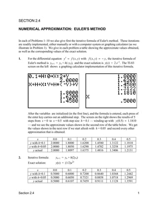
1. For the differential equation y′ = f ( x, y ) with f ( x, y ) = − y, the iterative formula of
Euler's method is yn+1 = yn + h(−yn), and the exact solution is y(x) = 2 e−x. The TI-83
screen on the left shows a graphing calculator implementation of this iterative formula.
After the variables are initialized (in the first line), and the formula is entered, each press of
the enter key carries out an additional step. The screen on the right shows the results of 5
steps from x = 0 to x = 0.5 with step size h = 0.1 — winding up with y (0.5) ≈ 1.1810
— and we see the approximate values shown in the second row of the table below. We get
the values shown in the next row if we start afresh with h = 0.05 and record every other
approximation that is obtained.
x 0.0 0.1 0.2 0.3 0.4 0.5
y with h=0.1 2.0000 1.8000 1.6200 1.4580 1.3122 1.1810
y with h=0.05 2.0000 1.8050 1.6290 1.4702 1.3258 1.1975
y actual 2.0000 1.8097 1.6375 1.4816 1.3406 1.2131
2. Iterative formula: yn+1 = yn + h(2yn)
Exact solution: y(x) = (1/2)e2x
x 0.0 0.1 0.2 0.3 0.4 0.5
y with h=0.1 0.5000 0.6000 0.7200 0.8640 1.0368 1.2442
y with h=0.05 0.5000 0.6050 0.7321 0.8858 1.0718 1.2969
y actual 0.5000 0.6107 0.7459 0.9111 1.1128 1.3591
Section 2.4 1

2. 3. Iterative formula: yn+1 = yn + h(yn + 1)
Exact solution: y(x) = 2ex − 1
x 0.0 0.1 0.2 0.3 0.4 0.5
y with h=0.1 1.0000 1.2000 1.4200 1.6620 1.9282 2.2210
y with h=0.05 1.0000 1.2050 1.4310 1.6802 1.9549 2.2578
y actual 1.0000 1.2103 1.4428 1.6997 1.9837 2.2974
4. Iterative formula: yn+1 = yn + h(xn − yn)
Exact solution: y(x) = 2e-x + x − 1
x 0.0 0.1 0.2 0.3 0.4 0.5
y with h=0.1 1.0000 0.9000 0.8200 0.7580 0.7122 0.6810
y with h=0.05 1.0000 0.9050 0.8290 0.7702 0.7268 0.6975
y actual 1.0000 0.9097 0.8375 0.7816 0.7406 0.7131
5. Iterative formula: yn+1 = yn + h(yn − xn − 1)
Exact solution: y(x) = 2 + x − ex
x 0.0 0.1 0.2 0.3 0.4 0.5
y with h=0.1 1.0000 1.0000 0.9900 0.9690 0.9359 0.8895
y with h=0.05 1.0000 0.9975 0.9845 0.9599 0.9225 0.8711
y actual 1.0000 0.9948 0.9786 0.9501 0.9082 0.8513
6. Iterative formula: yn+1 = yn + h(−2xnyn)
Exact solution: y(x) = 2 exp(−x2)
x 0.0 0.1 0.2 0.3 0.4 0.5
y with h=0.1 2.0000 2.0000 1.9600 1.8816 1.7687 1.6272
y with h=0.05 2.0000 1.9900 1.9406 1.8542 1.7356 1.5912
y actual 2.0000 1.9801 1.9216 1.8279 1.7043 1.5576
2
7. Iterative formula: yn+1 = yn + h(−3xn yn)
Exact solution: y(x) = 3 exp(−x3)
x 0.0 0.1 0.2 0.3 0.4 0.5
y with h=0.1 3.0000 3.0000 2.9910 2.9551 2.8753 2.7373
y with h=0.05 3.0000 2.9989 2.9843 2.9386 2.8456 2.6930
y actual 3.0000 2.9970 2.9761 2.9201 2.8140 2.6475
Section 2.4 2

3. 8. Iterative formula: yn+1 = yn + h exp(−yn)
Exact solution: y(x) = ln(x + 1)
x 0.0 0.1 0.2 0.3 0.4 0.5
y with h=0.1 0.0000 0.1000 0.1905 0.2731 0.3493 0.4198
y with h=0.05 0.0000 0.0976 0.1863 0.2676 0.3427 0.4124
y actual 0.0000 0.0953 0.1823 0.2624 0.3365 0.4055
2
9. Iterative formula: yn+1 = yn + h(1 + yn )/4
Exact solution: y(x) = tan[(x + π)/4]
x 0.0 0.1 0.2 0.3 0.4 0.5
y with h=0.1 1.0000 1.0500 1.1026 1.1580 1.2165 1.2785
y with h=0.05 1.0000 1.0506 1.1039 1.1602 1.2197 1.2828
y actual 1.0000 1.0513 1.1054 1.1625 1.2231 1.2874
2
10. Iterative formula: yn+1 = yn + h(2xnyn )
Exact solution: y(x) = 1/(1 − x2)
x 0.0 0.1 0.2 0.3 0.4 0.5
y with h=0.1 1.0000 1.0000 1.0200 1.0616 1.1292 1.2313
y with h=0.05 1.0000 1.0050 1.0306 1.0795 1.1579 1.2776
y actual 1.0000 1.0101 1.0417 1.0989 1.1905 1.3333
The tables of approximate and actual values called for in Problems 11–16 were produced using the
following MATLAB script (appropriately altered for each problem).
% Section 2.4, Problems 11-16
x0 = 0; y0 = 1;
% first run:
h = 0.01;
x = x0; y = y0; y1 = y0;
for n = 1:100
y = y + h*(y-2);
y1 = [y1,y];
x = x + h;
end
% second run:
h = 0.005;
x = x0; y = y0; y2 = y0;
for n = 1:200
y = y + h*(y-2);
y2 = [y2,y];
x = x + h;
end
Section 2.4 3

4. % exact values
x = x0 : 0.2 : x0+1;
ye = 2 - exp(x);
% display table
ya = y2(1:40:201);
err = 100*(ye-ya)./ye;
[x; y1(1:20:101); ya; ye; err]
11. The iterative formula of Euler's method is yn+1 = yn + h(yn − 2), and the exact solution is
y(x) = 2 − ex. The resulting table of approximate and actual values is
x 0.0 0.2 0.4 0.6 0.8 1.0
y ( h=0.01) 1.0000 0.7798 0.5111 0.1833 –0.2167 –0.7048
y (h=0.005) 1.0000 0.7792 0.5097 0.1806 –0.2211 –0.7115
y actual 1.0000 0.7786 0.5082 0.1779 –0.2255 –0.7183
error 0% –0.08% –0.29% –1.53% 1.97% 0.94%
12. Iterative formula: yn+1 = yn + h(yn − 1)2 /2
Exact solution: y(x) = 1 + 2/(2 − x)
x 0.0 0.2 0.4 0.6 0.8 1.0
y ( h=0.01) 2.0000 2.1105 2.2483 2.4250 2.6597 2.9864
y (h=0.005) 2.0000 2.1108 2.2491 2.4268 2.6597 2.9931
y actual 2.0000 2.1111 2.2500 2.4286 2.6597 3.0000
error 0% 0.02% 0.04% 0.07% 0.13% 0.23%
3
13. Iterative formula: yn+1 = yn + 2hxn /yn
Exact solution: y(x) = (8 + x4)1/2
x 1.0 1.2 1.4 1.6 1.8 2.0
y ( h=0.01) 3.0000 3.1718 3.4368 3.8084 4.2924 4.8890
y (h=0.005) 3.0000 3.1729 3.4390 3.8117 4.2967 4.8940
y actual 3.0000 3.1739 3.4412 3.8149 4.3009 4.8990
error 0% 0.03% 0.06% 0.09% 0.10% 0.10%
2
14. Iterative formula: yn+1 = yn + hyn /xn
Exact solution: y(x) = 1/(1 − ln x)
x 1.0 1.2 1.4 1.6 1.8 2.0
y ( h=0.01) 1.0000 1.2215 1.5026 1.8761 2.4020 3.2031
y (h=0.005) 1.0000 1.2222 1.5048 1.8814 2.4138 3.2304
y actual 1.0000 1.2230 1.5071 1.8868 2.4259 3.2589
error 0% 0.06% 0.15% 0.29% 0.50% 0.87%
Section 2.4 4

5. 15. Iterative formula: yn+1 = yn + h(3 − 2yn /xn)
Exact solution: y(x) = x + 4/x2
x 2.0 2.2 2.4 2.6 2.8 3.0
y ( h=0.01) 3.0000 3.0253 3.0927 3.1897 3.3080 3.4422
y (h=0.005) 3.0000 3.0259 3.0936 3.1907 3.3091 3.4433
y actual 3.0000 3.0264 3.0944 3.1917 3.3102 3.4444
error 0% 0.019% 0.028% 0.032% 0.033% 0.032%
5 2
16. Iterative formula: yn+1 = yn + 2hxn /yn
Exact solution: y(x) = (x6 − 37)1/3
x 2.0 2.2 2.4 2.6 2.8 3.0
y ( h=0.01) 3.0000 4.2476 5.3650 6.4805 7.6343 8.8440
y (h=0.005) 3.0000 4.2452 5.3631 6.4795 7.6341 8.8445
y actual 3.0000 4.2429 5.3613 6.4786 7.6340 8.8451
error 0% –0.056% –0.034% –0.015% 0.002% 0.006%
The tables of approximate values called for in Problems 17-24 were produced using a MATLAB
script similar to the one listed preceding the Problem 11 solution above.
17.
x 0.0 0.2 0.4 0.6 0.8 1.0
y ( h=0.1) 0.0000 0.0010 0.0140 0.0551 0.1413 0.2925
y (h=0.02) 0.0000 0.0023 0.0198 0.0688 0.1672 0.3379
y (h=0.004) 0.0000 0.0026 0.0210 0.0717 0.1727 0.3477
y (h=0.0008) 0.0000 0.0027 0.0213 0.0723 0.1738 0.3497
These data that y(1) ≈ 0.35, in contrast with Example 4 in the text, where the initial
condition is y(0) = 1.
In Problems 18−24 we give only the final approximate values of y obtained using Euler's method
with step sizes h = 0.1, h = 0.02, h = 0.004, and h = 0.0008.
18. With x0 = 0 and y0 = 1, the approximate values of y(2) obtained are:
h 0.1 0.02 0.004 0.0008
y 1.6680 1.6771 1.6790 1.6794
19. With x0 = 0 and y0 = 1, the approximate values of y(2) obtained are:
h 0.1 0.02 0.004 0.0008
y 6.1831 6.3653 6.4022 6.4096
Section 2.4 5

6. 20. With x0 = 0 and y0 = −1, the approximate values of y(2) obtained are:
h 0.1 0.02 0.004 0.0008
y −1.3792 −1.2843 −1.2649 −1.2610
21. With x0 = 1 and y0 = 2, the approximate values of y(2) obtained are:
h 0.1 0.02 0.004 0.0008
y 2.8508 2.8681 2.8716 2.8723
22. With x0 = 0 and y0 = 1, the approximate values of y(2) obtained are:
h 0.1 0.02 0.004 0.0008
y 6.9879 7.2601 7.3154 7.3264
23. With x0 = 0 and y0 = 0, the approximate values of y(1) obtained are:
h 0.1 0.02 0.004 0.0008
y 1.2262 1.2300 1.2306 1.2307
24. With x0 = −1 and y0 = 1, the approximate values of y(1) obtained are:
h 0.1 0.02 0.004 0.0008
y 0.9585 0.9918 0.9984 0.9997
25. With step sizes h = 0.15, h = 0.03, and h = 0.006 we get the following results:
y with y with y with
x h=0.15 h=0.03 h=0.006
−1.0 1.0000 1.0000 1.0000
−0.7 1.0472 1.0512 1.0521
−0.4 1.1213 1.1358 1.1390
−0.1 1.2826 1.3612 1.3835
+0.2 0.8900 1.4711 0.8210
+0.5 0.7460 1.2808 0.7192
While the values for h = 0.15 alone are not conclusive, a comparison of the values of y
for all three step sizes with x > 0 suggests some anomaly in the transition from negative to
positive values of x.
26. With step sizes h = 0.1 and h = 0.01 we get the following results:
y with y with
x h = 0.1 h = 0.01
Section 2.4 6

7. 0.0 0.0000 0.0000
0.1 0.0000 0.0003
0.2 0.0010 0.0025
0.3 0.0050 0.0086
⋅ ⋅ ⋅
⋅ ⋅ ⋅
⋅ ⋅ ⋅
1.8 2.8200 4.3308
1.9 3.9393 7.9425
2.0 5.8521 28.3926
Clearly there is some difficulty near x = 2.
27. With step sizes h = 0.1 and h = 0.01 we get the following results:
y with y with
x h = 0.1 h = 0.01
0.0 1.0000 1.0000
0.1 1.2000 1.2200
0.2 1.4428 1.4967
⋅ ⋅ ⋅
⋅ ⋅ ⋅
⋅ ⋅ ⋅
0.7 4.3460 6.4643
0.8 5.8670 11.8425
0.9 8.3349 39.5010
Clearly there is some difficulty near x = 0.9.
Section 2.4 7