
Recomendados
Recomendados
Mais conteúdo relacionado
Mais procurados
Mais procurados (20)
Semelhante a High-order Numerical Methods for Predictive Science
Semelhante a High-order Numerical Methods for Predictive Science (20)
Último
Último (20)
High-order Numerical Methods for Predictive Science
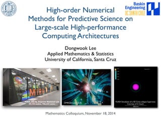
- 1. High-order Numerical Methods for Predictive Science on Large-scale High-performance Computing Architectures Dongwook Lee Applied Mathematics & Statistics University of California, Santa Cruz Mathematics Colloquium, November 18, 2014 FLASH Simulation of a 3D Core-collapse Supernova Courtesy of S. Couch MIRA, BG/Q, Argonne National Lab 49,152 nodes, 786,432 cores OMEGA Laser (US)
- 2. Cyclic Relationship Theory Experiment Scientific Computation validation verification
- 3. Example: Supersonic Airflow Theory Experiment Simulation
- 4. Topics for Today 1. High Performance Computing 2. Ideas on Numerical Methods 3. Validation & Predictive Science
- 5. First Episode 1. High Performance Computing 2. Ideas on Numerical Methods 3. Validation & Predictive Science
- 6. High Performance Computing (HPC) ‣To solve large problems in science, engineering, or business ‣Modern HPC architectures have ▪ increasing number of cores ▪ declining memory/core ‣This trend will continue for the foreseeable future
- 7. High Performance Computing (HPC) ‣This tension between computation & memory brings a paradigm shift in numerical algorithms for HPC ‣To enable scientific computing on HPC architectures: ▪ efficient parallel computing, (e.g., data parallelism, task parallelism, MPI, multi-threading, GPU accelerator, etc.) ▪ better numerical algorithms for HPC
- 8. Numerical Algorithms for HPC ‣Numerical algorithms should conform to the abundance of computing power and the scarcity of memory. ‣But… ▪ without losing solution accuracy. ▪ with maintaining maximum solution stability. ▪ with faster convergence to a “correct” solution.
- 9. High-Order Numerical Algorithms ‣ A good solution to this is to use high-order algorithms. ‣ They provide more accurate numerical solutions using ▪ less grid points (=memory save). ▪ higher-order mathematical approximations (promoting more floating point operations, or computation). ▪ faster convergence to solution.
- 10. Large Scale Astrophysics Codes ▪FLASH (Flash group, U of Chicago) Future HPC ▪ PLUTO (Mignone, U of Torino), ▪ CHOMBO (Colella, LBL) ▪ CASTRO (Almgren, Woosley, LBL, UCSC) ▪ MAESTRO (Zingale, Almgren, SUNY, LBL) ▪ ENZO (Bryan, Norman, Abel, Enzo group) ▪ BATS-R-US (CSEM, U of Michigan) ▪ RAMSES (Teyssier, CEA) Peta- Scale ▪ Current HPC CHARM (Miniati, ETH) ▪ AMRVAC (Toth, Keppens, CPA, K.U.Leuven) ▪ ATHENA (Stone, Princeton) ▪ ORION (Klein, McKee, U of Berkeley) ▪ ASTROBear (Frank, U of Rochester) ▪ ART (Kravtsov, Klypin, U of Chicago) ▪ NIRVANA (Ziegler, Leibniz-Institut für Astrophysik Potsdam), and others Giga- Scale Current Laptop/Desktop ?
- 11. The FLASH Code ‣FLASH is is free, open source code for astrophysics and HEDP. ▪ modular, multi-physics, adaptive mesh refinement (AMR), parallel (MPI & OpenMP), finite-volume Eulerian compressible code for solving hydrodynamics and MHD ▪ professionally software engineered and maintained (daily regression test suite, code verification/validation), inline/online documentation ▪ 8500 downloads, 1500 authors, 1000 papers ▪ FLASH can run on various platforms from laptops to supercomputing (peta-scale) systems such as IBM BG/P and BG/Q.
- 12. Scientific Simulations using FLASH cosmological cluster formation supersonic MHD turbulence Type Ia SN RT CCSN ram pressure stripping laser slab rigid body structure Accretion Torus LULI/Vulcan experiments: B-field generation/amplification
- 13. Parallel Computing ‣ Adaptive Mesh Refinement (w/ Paramesh) ▪conventional parallelism via MPI (Message Passing Interface) ▪domain decomposition distributed over multiple processor units ▪distributed memory (cf. shared memory) Single block uniform grid octree-based block AMR patch-based AMR
- 14. Parallelization, Optimization & Speedup 16 GB/node 16 cores/node 4 threads/core
- 15. Parallelization, Optimization & Speedup ‣Multi-threading (shared memory) using OpenMP directives ▪more parallel computing on BG/Q using hardware threads on a core ▪ 16 cores/node, 4 threads/core thread block list thread within block ▪ 5 leaf blocks in a single MPI rank ▪ 2 threads/core (or 2 threads/rank)
- 16. FLASH Scaling Test on BG/Q RTFlame, strong scaling: 4 threads/rank CCSN, weak scaling: 8 threads/rank VESTA: 2 racks 1024 nodes/rack 10 8 6 4 2 MIRA: 48 racks 1024 nodes/rack BG/Q: 16 cores/node 4 threads/core 16GB/core 512 (4k) 1024 (8k) 2048 (16k) 4096 (32k) 8192 (64k) 16384 (128k) 25 20 15 10 5 32768 (256k) Mira nodes (ranks), 8 threads/rank 0 108 core hours/zone/step 0 107 core hours/zone/IO write Total evolution MHD Gravity Grid IO (1 write) ⌫-Leakage Ideal
- 17. Second Episode 1. High Performance Computing 2. Ideas on Numerical Methods 3. Validation Predictive Science
- 18. Scientific Tasks Science Problem (IC, BC, ODE/PDE) Simulator (code, computer) Results (Validation, verification, analysis)
- 19. 1. Mathematical Models Hydrodynamics (gas dynamics) @⇢ @t + r · (⇢v) = 0 mass eqn @⇢v @t + r · (⇢vv) + rP = ⇢g momentum eqn @⇢E @t + r · [(⇢E + P)v] = ⇢v · g total energy eqn P = (! 1)⇢✏ E = ✏ + 1 2|v|2 @⇢✏ @t + r · [(⇢✏ + P)v] − v · rP = 0 Equation of State
- 20. 2. Mathematical Models Magnetohydrodynamics (MHD) @⇢ @t + r · (⇢v) = 0 mass eqn @⇢v @t + r · (⇢vv − BB) + rP⇤ = ⇢g + r · ⌧ momentum eqn @⇢E @t + r · [v(⇢E + P⇤) − B(v · B)] = ⇢g · v + r · (v · ⌧ + $rT) + r · (B ⇥ (⌘r⇥B)) total energy eqn @B @t + r · (vB − Bv) = −r ⇥ (⌘r⇥B) induction eqn P⇤ = p + B2 2 E = v2 2 + ✏ + B2 2⇢ Equation of State ⌧ = μ[(rv) + (rv)T − 2 3 solenodidal constraint (r · v)I] viscosityr · B = 0
- 21. 3. Mathematical Models HEDP: Separate energy eqns for ion, electron, radiation (“3-temperature, or 3T”) @ @t (⇢✏ion) + r · (⇢✏ionv) + Pionr · v = ⇢ cv,ele ⌧ei (Tele − Tion) ion energy @ @t (⇢✏ele) + r · (⇢✏elev) + Peler · v = ⇢ cv,ele ⌧ei (Tion − Tele)−r· qele + Qabs − Qemis + Qlas electron energy @ @t (⇢✏rad) + r · (⇢✏radv) + Pradr · v = r · qrad − Qabs + Qemis radiation energy ✏tot = ✏ion + ✏ele + ✏rad Ptot, Tion, Tele, Trad = EoS(⇢, ✏ion, ✏ele, ✏rad) 3T EoS Compare 3T with a simple 1T EoS! @ @t (⇢✏tot) + r · (⇢✏totv) + Ptotr · v = 0 Ptot = EoS(⇢, ✏tot) Tion = Tele = Trad, or Tele = Tion, Trad = 0
- 22. Discretization Approaches ‣Finite Volume (FV) ▪shock capturing, compressible flows, structured/unstructured grids ▪hard to achieve high-order (higher than 2nd order) ‣Finite Difference (FD) ▪smooth flows, incompressible, high-order methods ▪non-conservative, simple geometry ‣Finite Element (FE) ▪arbitrary geometry, basis functions, continuous solutions ▪hard coding, problems at strong gradients ‣Spectral Element (SE) ‣Discontinuous Galerkin (DG)
- 23. Finite Volume Formulations @U @t + @F @x + @G @y + @H @z = 0 @U @t + r · Flux(U) = 0 ‣ Conservation laws (mass, momentum, energy) ‣ Highly compressible flows with shocks and discontinuities ‣ Differential (smooth) form of PDEs (e.g., FD) becomes invalid ‣ Integral form of PDEs relaxes the smoothness assumptions and seek for weak solutions over control volumes and boundaries ‣ Basics of FV (in 1D): U i+1 n x t Un+1 i Un i Un i1 tn+1 tn Fn i1/2 Fn i+1/2 or
- 24. Finite Volume Formulations ‣ Integral form of PDE: Z xi+1/2 xi1/2 u(x, tn+1)dx Z xi+1/2 xi1/2 u(x, tn)dx = Z tn+1 tn f(u(xi1/2, t))dt Z tn+1 tn f(u(xi+1/2, t))dt ‣ Volume averaged, cell-centered quantity time averaged flux: Un i = 1 x Z xi+1/2 xi1/2 and f(u(xi1/2, t))dt u(x, tn)dx Fn i1/2 = ‣ Finite wave speed in hyperbolic system: 1 t Z tn+1 tn Fn i1/2 = F(Un i ) * High-order reconstruction in space time i1, Un * Riemann problem at each cell-interface, i-1/2 ‣ General discrete difference equation in conservation form in 1D: Un+1 i = Un i t x (Fn i+1/2 Fn i1/2)
- 25. Riemann Problem Godunov Method ‣The Riemann problem: ‣Two cases: PDEs: Ut + AUx = 0,−1 x 1, t 0 IC : U(x, t = 0) = U0(x) = ( UL if x 0, UR if x 0. Shock solution Rarefaction solution
- 26. A Discrete World of FV U(x, tn) xi1 xi xi+1
- 27. A Discrete World of FV piecewise polynomial reconstruction on each cell u(xi, tn) = Pi(x), x 2 (xi1/2, xi1/2) xi1 xi xi+1 uR = Pi(xi+1/2) uL = Pi+1(xi+1/2)
- 28. A Discrete World of FV At each interface we solve a RP and obtain Fi+1/2 xi1 xi xi+1
- 29. A Discrete World of FV We are ready to advance our solution in time and get new volume-averaged states Un+1 i = Un i t x ⇣ F⇤ i+1/2 F⇤ i−1/2 ⌘
- 30. High-Order Polynomial Reconstruction PLM PPM FOG • Godunov’s order-barrier theorem (1959) • Monotonicity-preserving advection schemes are at most first-order! (Oh no…) • Only true for linear PDE theory (YES!) • High-order “polynomial” schemes became available using non-linear slope limiters (70’s and 80’s: Boris, van Leer, Zalesak, Colella, Harten, Shu, Engquist, etc) • Can’t avoid oscillations completely (non-TVD) • Instability grows (numerical INSTABILITY!)
- 31. Low vs. High order Reconstructions
- 32. Traditional High-Order Schemes ‣ Traditional approaches to get Nth high-order schemes take (N-1)th degree polynomial for interpolation/reconstruction ▪only for normal direction (e.g., PLM, PPM, ENO, WENO, etc) ▪with monotonicity controls (e.g., slope limiters, artificial viscosity) ‣ High-order in FV is tricky (when compared to FD) ▪volume-averaged quantities (quadrature rules) ▪preserving conservation w/o losing accuracy ▪higher the order, larger the stencil ▪high-order temporal update (ODE solvers, e.g., RK3, RK4, etc.) 2D stencil for 2nd order PLM 2D stencil for 3rd order PPM
- 33. Stability, Consistency and Convergence ‣Lax Equivalence Theorem (for linear problem, P. Lax, 1956) ▪The only convergent schemes are those that are both consistent and stable. ▪Hard to show that the numerical solution converges to the original solution of PDE; relatively easy to show consistency and stability of numerical schemes ‣In practice, non-linear problems adopts the linear theory as guidance. ▪code verification (code-to-code comparison) ▪code validation (code-to-experiment, code-to-analytical solution comparisons) ▪self-convergence test over grid resolutions (a good measurement for numerical accuracy)
- 34. Shu-Osher Problem:1D Mach 3 Shock
- 36. Circularly Polarized Alfven Wave ▪A CPAW problem propagates smoothly varying oscillations of the transverse components of velocity and magnetic field. ▪The initial condition is the exact nonlinear solutions of the MHD equations. ▪The decay of the max of Vz and Bz is solely due to numerical dissipation: direct measurement of numerical diffusion (Ryu, Jones Frank, ApJ, 1995; Toth 2000, Del Zanna et al. 2001; Gardiner Stone 2005, 2008). A. Mignone et al. / Journal of Computational Physics 229 (2010) 5896–5920 5907 Source: Mignone Tzeferacos, 2010, JCP Fig. A.3. Long term decay of circularly polarized Alfvén waves after 16.5 time units, corresponding to ) 100 wave periods. In the left panel, we plot the maximum value of the vertical component of velocity as a function of time for the WENO $ Z (solid line) and WENO + 3 (dashed line) schemes. For
- 37. Performance Comparison L1 norm error avg. comp. time / step 0.221 (x5/3)sec 38.4 sec 32 256 Source: Mignone Tzeferacos, 2010, JCP ▪PPM (overall 2nd order): 2h42m50s ▪MP5 (5th order): 15s(x5/3)=25s ▪More computational work less memory ▪Better suited for HPC ▪Easier in FD; harder in FV ▪High-orders schemes are better in preserving solution accuracy on AMR.
- 38. Truncation Errors at Fine-Coarse Boundary Ff,L i1/2,j+1/4 DF = (i⇤, j) i1/2,j Ff,L i1/2,j1/4 Fc,R U t 1 x = 1 x + r · F = TE = h Fc,R i+1/2,j − 1 2 (Ff,L i1/2,j+1/4 + Ff,L h F # (i + 1/2)x, jy $ − F # (i − 1/2)x, jy ( O(h) at F/C boundary O(h2) otherwise i1/2,j1/4) i $ + O(y2) ✓Any 2nd order Scheme becomes 1st order at fine-coarse boundaries. ✓The deeper AMR level, the worse truncation errors accumulated and solutions will become 1st order almost everywhere if grid pattern changes frequently. ✓High-order scheme is NOT just an option! (see papers by Colella et al.) i = @F @x + O(h), assuming x ⇡ y(= h)
- 39. Multidimensional Formulation ‣ 2D discrete difference equation in conservation form: Un+1 i,j = Un i,j t x (Fn i+1/2,j Fn ‣ Two different approaches: ‣ directionally “split” formulation i1/2,j) t y (Gn i,j+1/2 Gn i,j1/2) ‣ update each spatial direction separately, easy to implement, robust ‣ always good? ‣ directionally “unsplit” formulation ‣ update both spatial directions at the same time, harder to implement ‣ you gain improved extra bonus (i.e., stability) from what you pay for!
- 40. Unsplit FV Formulation ‣ 2D discrete difference equation in conservation form: Un+1 i,j = Un i,j ut x [Un i,j Un i1,j ] vt y [Un i,j1] Un+1 i,j Un i,j = Un i,j ut x [Un i,j Un i1,j ] vt y [Un i,j Un i,j1] + t2 2 n u x ⇥ v y (Un i,j Un i,j1) v y (Un i1,j Un i1,j1) ⇤ + v y ⇥ v y (Un i,j Un i1,j) v y (Un i,j1 Un i1,j1) ⇤o Extra cost for corner coupling! (a) 1st order donor cell (i, j) Un+1 i,j = Un i,j t x (Fn i+1/2,j Fn i1/2,j) t y (Gn i,j+1/2 Gn i,j1/2) (b) 2nd order corner-transport-upwind (CTU) (i, j)
- 41. Unsplit FV Formulation ‣ 2D discrete difference equation in conservation form: Un+1 i,j = Un i,j t x (Fn i+1/2,j Fn i1/2,j) t y (Gn i,j+1/2 Gn i,j1/2) (a) 1st order donor cell ut x (i, j) + vt y (b) 2nd order corner-transport-upwind (CTU) 1 max ⇣ (i, j) ut x , vt y ⌘ 1 Smaller stability region Gain: Extended stability region
- 42. Unsplit vs. Split ✓Single-mode RT instability (Almgren et al. ApJ, 2010) ✓Split solver: High-wavenumber instabilities grow due to experiencing high compression and expansion in each directional sweep. ✓Unsplit solver: High-wavenumber instabilities are suppressed and do not grow. ✓ For MHD, it is more crucial to use unsplit in order to preserve divergence-free solenoidal constraint (Lee Deane, 2009; Lee, 2013): Split PPM Unsplit PPM r · B = @Bx @x + @By @y + @Bz @z = 0
- 43. Unsplit vs. Split unsplit PPM split PPM
- 45. Last Episode 1. High Performance Computing 2. Ideas on Numerical Methods 3. Validation Predictive Science
- 46. In Collaboration with U of Chicago: D. Q. Lamb P. Tzeferacos N. Flocke C. Graziani K. Weide U of Oxford: G. Gregori J. Meinecke
- 47. To Investigate B-field in the Universe • In the universe, shocks are driven when two or more giant galaxy clusters are merging together by gravitational collapsing. • Mass accretion onto these clusters generate high Mach number shocks. • These shocks can form a tiny “seed” magnetic fields which can then be amplified by turbulent dynamo processes. Filaments Clusters Voids Expanding Shocks Courtesy of F. Miniati (ETH) Courtesy of A. Kravtsov U of Chicago
- 48. Shock Waves In SNR Cool Ejecta Shocked Ejecta due to Reverse Shocks • Narrow X-ray filaments (~ parsec in width) at the outer shock rim are produced by synchrotron radiation from ultra-relativistic electrons. • The B-fields in the outer region ~ 100μG or more. Inner Region Forward Shock Wave Circumstellar Gas Outer Region • The interior of the SNR Cassiopeia A contains a disordered shell of radio synchrotron emission by giga-electronvolt electrons. •The inferred magnetic field in these radio knots is a few milli-gauss, about 100 times larger than the surrounding interstellar gas.
- 49. Biermann Battery Mechanism • The origin of the magnetic fields in the universe is still not yet fully understood. • Generalized Ohm’s law: The BBT is the mostly widely invoked mechanism to produce B fields from unmagnetized plasma condition , where J = r ⇥ B (1) dynamo term (2) resistive term (3) Hall term (4) Biermann battery term (BBT) E =− u ⇥ B c + ⌘J + J ⇥ B cnee − rpe nee
- 50. Takeaway @B @t BBT = crPe ⇥rne qen2e • BBT generates B fields when gradients of electron pressure and density are not aligned. • BBT is zero in 1D (or symmetric) flow or at spherical shocks. • BBT becomes non-zero when symmetry is broken, and two gradients are not aligned to each other, that is, at downstream of BBT = 0 BBT≠0 asymmetric shock. We use laser to drive asymmetric shocks! Please see our new study on BBT: Graziani et al., submitted to ApJ, 2014
- 51. Magnetic Fields in HEDP Tzeferacos et al., HEDP, 2014, Accepted Meinecke et al., Nature Physics, 2014
- 52. Investigating B-field in the Universe 300$J$1ns$ 3cm$ $2ω$ 3,axis$coils$ Ar$(1atm)$ 4cm$ Carbon$rod$ 4cm$ In collaboration with the research teams in U of Chicago Oxford Univ. Experimental Configuration
- 53. Investigating B-field in the Universe In collaboration with the research teams in U of Chicago Oxford Univ. 3D Simulation
- 54. Validation Predictive Science • We used five Vulcan laser shots (280-300J) to calibrate the fraction of the laser energy deposited in the carbon rod target. • With the calibrated amount of laser energy deposition we predicted the shock radius of six laser shots with energies ranging from 200-343J. breakout)shock) material) discon2nuity) shock) shock)generated)B laser5target)B t=50ns Laserenergyrangeusedtocalibrateε
- 55. Validation Predictive Science Experimental,data, FLASH, shock,radius,(mm), t,(μs), Meinecke et al., Nature Physics, 2-14
- 56. Summary ▪Novel ideas of numerical algorithms can play the key fundamental role in many areas in modern science. ▪Computational mathematics is one of the corner stone research areas that can provide major predictive scientific tools. ▪Numerical simulations can help designing better scientific directions in wide ranges of research applications, especially in physical science and engineering.
- 57. Thanks! Questions? Dongwook Lee: dlee79@ucsc.edu ams.soe.ucsc.edu/people/dongwook FLASH: www.flash.uchicago.edu
- 59. Relavant Questions ‣ What is scientific computing? ‣ How do we want to use computer for it? ‣ What should we do in order to use computing resources in a better way? ‣ Can numerical algorithms and computational mathematics improve computations? ‣ High-performance computing: petascale (or exascale ?)
- 60. Various Reconstruction 1st 2nd 3rd 5th 200 cells 1st on 400 cells 1st on 800 cells 1st + HLL 1st + HLLC 1st + Roe 200 cells
- 61. Low-Order vs. High-Order 1st Order High-Order Ref. Soln 1st order: 3200 cells (50 MB), 160 sec, 3828 steps vs. High-order: 200 cells (10 MB), 9 sec, 266 steps