Recomendados

Recomendados
Mais conteúdo relacionado
Mais procurados
Mais procurados (20)
Semelhante a Correspondence Analysis for Discrete Multivariate Statistics
Semelhante a Correspondence Analysis for Discrete Multivariate Statistics (20)
Mais de dessybudiyanti
Mais de dessybudiyanti (20)
Último
Último (20)
Correspondence Analysis for Discrete Multivariate Statistics
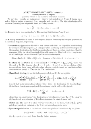
- 1. MULTIVARIATE STATISTICS, Lesson 11. Correspondence Analysis (Discrete version of the canonical correlation analysis) We have two – usually not independent – discrete (categorical) r.v.’s X and Y taking on n and m different values, respectively (e.g., hair-color and eye-color). The joint distribution R is estimated from the joint frequencies based on N observations: fij rij = (i = 1, . . . , n; j = 1, . . . , m). N Let R denote the n × m matrix of rij ’s. The marginal distributions P and Q are: pi = ri. (i = 1, . . . , n) and qj = r.j (j = 1, . . . , m). Let P and Q denote the n × n and m × m diagonal matrices containing the marginal probabilities in their main diagonals, respectively. • Problem: to approximate the table R with a lower rank table. For tis purpose we are looking for correspondence factor pairs αl , βl taking on values and having unit variance with respect to the marginal distributions, further being maximally correlated on certain constraints. ER αβ is maximum (1) for the trivial (constantly 1) variable pair α1 , β1 . Then for k = 2, . . . , min{n, m} we are looking for the maximum of ER αβ on the constraints that EP α = EQ β = 0, D2 α = D2 β = 1, P Q Cov P ααi = Cov Q ββi = 0 (i = 1, . . . , k − 1). • Solution: by the SVD of the n × m matrix B = P−1/2 RQ−1/2 = r sl vl uT , where r is l=1 l the rank of R. The singular values 1 = s1 ≥ s2 ≥ · · · ≥ sr > 0 are the correlations of the correspondence factor pairs, while the values taken on by the k-th pair are coordinates of the correspondence vectors P−1/2 vk and Q−1/2 uk , respectively. • Hypothesis testing: to test the independence of X and Y , the test statistic n m n m 2 r (rij − pi qj )2 rij 2 t=N =N − 1 = N B − B1 F =N s2 l i=1 j=1 pi qj i=1 j=1 pi qj l=2 is used, that under independence follows χ2 ((n − 1)(m − 1))-distribution. To thest the hypo- thesis that a k-rank approximation of the contingency table suffices, the statistic r N B− Bk 2 F =N s2 , l k = 1, . . . , r − 1 l=k+1 k should take on small values” (its distribution is yet unknown), where Bk = l=1 sl vl uT is l ” the best k-rank approximation of B in Frobenius norm (in spectral norm, too). k • Definition: The above t is called total correspondence of the table, while N l=2 s2 /t is l called correspondence explained by the first k correspondence factor pairs. • Spacial representation of the row and column categories in k dimension: by the points (α1 (i), α2 (i), . . . , αk (i)) and (β1 (j), β2 (j), . . . , βk (j)) (i = 1, . . . , n; j = 1, . . . , m). Store them for further analysis.