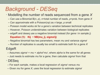
1. Background - DESeq
• Modelling the number of reads sequenced from a gene X
– Can use a Binomial B(n, p), n=total number of reads, p=prob. from gene X
– Can approximate with a Poisson(np) as n large, p small
– Poisson model works ok for a gene’s variation between technical replicates
– However, Poisson understimates variation between biological replicates
– edgeR and deseq use a negative binomial instead (for gene i in sample j)
Equation (1): Kij ~ NB(mu_ij, sigma2
ij)
– Negative binomial has two parameters, mean mu and variance sigma2
– Number of replicates is usually too small to estimate both for a gene X
EdgeR
– Assumes sigma2
= mu + alpha*mu2
, where alpha is the same for all genes
– Just needs to estimate mu for a gene, then calculate sigma2
from that
• DESeq
– For each sample, makes a local regression of sigma2
versus mu
– Given mu for gene X, uses the local regression to estimate sigma2

2. Results & Discussion
• DESeq’s model - makes three assumptions
– Equation (2): mu_ij = qi,rho(j) * sj
mu_ij = expected value of mean count (no. reads) for gene i in sample j
qi,rho(j) = proportional to concentration of fragments from gene i in sample j
sj = coverage (sampling depth) of library j
– Equation (3): sigma2
_ij = mu_ij + sj2
* vi,rho(j)
sigma2_ij = variance of no. reads for gene i in sample j
mu_ij = variance due to Poisson model (technical variation) = “shot noise”
sj2
* vi,rho(j) = variance due to biological variation(?) = “raw variance”
– Equation (4): vi,rho(j) = vrho ( qi,rho(j) )
ie. vi,rho(j) is a function of qi,rho(j)
So we can make a regression of vi,rho(j) against qi,rho(j) for lots of genes (i)
Then estimate vi,rho(j) for gene X, based on qi,rho(j) and the regression line

3. • DESeq’s model – estimating parameters
– sj : coverage (sampling depth) of library j
The total number of reads in library j is not a good measure of depth.
Instead, take the median (over all genes) of the ratios of observed counts:
Equation (5): sj = median_over_i ( kij / [ Sum_over_v kiv ]^(1/m) ] )
– qi,rho(j) = “expression strength” parameter for gene i in condition rho
Proportional to concentration of fragments from gene i in sample j.
Use the average of countsfrom samples j for condition rho:
Equation (6): qi,rho = 1/m_rho * Sum_over_j (kij / sj)
– vrho = function describing how vi,rho(j) depends on qi,rho(j)
Estimate the sample variance for each gene i, wi(rho) (Equation 7)
Fit a local regression line to wi(rho) versus qi(rho)
For a particular qi(rho) value, predict w=wi(rho) from the regression line
Also calculate zi(rho) for gene i (Equation 8)
Then use v = w – zi(rho) as an unbiased estimate of the variance vi,rho for
gene i (Equation 9)

4. • DESeq’s model – testing for differential expression
– Null hypothesis: qiA = qiB
qiA = expression strength parameter for gene i in the samples of condition A,
mA = number of samples for condition A
– Test statistic: total counts in each condition
Equation (10): KiA = counts in condition A = Sum_over_A ( Kij)
– P-value for test of null hypothesis
Under the null hypothesis, can compute prob(KiA = a, KiB = b) = p(a,b)
Equation (11): P-value for observed count (kiA, kiB) =
Sum of probabilities p(a,b) where p(a,b)≤ p(kiA,kiB), a+b = kiA+kiB
Sum of probabilities p(a,b) where a+b = kiA+kiB
– Computing p(a,b) values
p(a,b) = Prob(KiA = a) * Prob(KiB = b), assuming samples are independent
KiA is the sum of mA NB-distributed variables
We approximate its distribution by a NB(mu, sigma) distribution
whose parameters mu, sigma are estimated using Equations 12,13,14

5. Applications
• Variance estimation
– Use RNA-seq data from fly embryos: ‘A’ and ‘B’ samples, 2 replicates each
Figure 1: estimated variances wi(rho) plotted against qi(rho) for fly sample A
Distance between orange and purple lines is noise due to biological sampling
regression
edgeR
“shot noise”
(technical
variation)

6. • Testing for differential expression
– Compared the 2 replicates for fly sample A
Figure 2: the empirical cumulative distribution functions of the P-values
The ECDF curve (blue line) should be below the diagonal (gray line)
Type I error is controlled by EdgeR & DESeq, but not a Poisson-based test
EdgeR has an excess of small P-values for low counts, but is more
conservative for high counts
DESeq
edgeR
Poisson
Low High All

7. • Testing for differential expression
– Compared fly A & B samples
Figure 3: obtained fold changes and P-values
The ability to detect differential expression depends on overall counts
The strong shot noise (technical variation) for low counts causes the testing
procedure to call only very high fold changes as significant
Red: significant p-value

8. • Comparison with EdgeR
– Ran edgeR with 4 settings:
(i) “Common-dispersion” or “tagwise-dispersion” modes for estimating variance
(ii) Size factors estimated by DESeq, or total number of reads
Results were very similar for the 4 settings
EdgeR’s single-value dispersion estimate of variance is lower than DESeq for
weakly expressed genes & higher for strongly expressed genes (Figure 1)
regression
edgeR
“shot noise”
(technical
variation)
As a result, EdgeR is anti-conservative for
lowly expressed genes, but more
conservative for strongly expressed genes

9. This biases the list of discoveries by EdgeR
Figure 4 shows that weakly expressed genes seem to be over-represented
Few genes with high average level are called differentially expressed by EdgeR
DESeq produced results which were more balanced over the dynamic range
All fly data
DESeq hits
EdgeR hits

10. • Working without replicates
– DESeq can work if there are no replicates in one or both conditions
If there are just replicates from one condition, fit regression line using that one
If there are no replicates, treat the samples as replicates to fit the regression
For neural cell data, variability between replicates ≈ variability bet. conditions
However, for fly data, variability between replicates << variability bet. conditions

11. • Variance-stabilising transformation (VST)
– Given a variance-mean regression, a VST transforms the values so the
variance is independent of the mean (Equation 15)
This yields (transformed) count values whose variances are approximately
the same throughout the dynamic range
This is useful for sample clustering, since clustering assumes all genes have
roughly the same variance
Figure 5 shows clustering for neural cell samples, using VST-transformed data

12. • ChIP-Seq data
– Compared HapMap IDs GM12878 and GM12891
DESeq does not give false positives when comparing replicates for 1 individual
Using a Poisson-based model, you would get many false positives
DESeq
Poisson
Same individual Different individuals

13. Summary
• A Poisson model underestimates the variance between
biological samples; this leads to false positives in differential
expression analyses
• A Negative Binomial distribution is much better
• This is especially true for highly expressed genes
• DESeq and EdgeR use the Negative Binomial
• However, DESeq estimates the sequencing depth differently
• Also DESeq estimates the variance for a gene by assuming
it has similar variance to genes of similiar expression level
• DESeq and EdgeR have similar sensitivity, but EdgeR calls a
greater number of weakly expressed genes as significant,
and fewer highly expressed genes as significant