2. 36 2 Vector and Tensor Analysis in Euclidean Space
3. Scalar product of two vector- or tensor-valued functions:
d
dt
Œx .t/ y .t/ D
dx
dt
y .t/ C x .t/
dy
dt
; (2.6)
d
dt
ŒA .t/ W B .t/ D
dA
dt
W B .t/ C A .t/ W
dB
dt
: (2.7)
4. Tensor product of two vector-valued functions:
d
dt
Œx .t/ ˝ y .t/ D
dx
dt
˝ y .t/ C x .t/ ˝
dy
dt
: (2.8)
5. Composition of two tensor-valued functions:
d
dt
ŒA .t/ B .t/ D
dA
dt
B .t/ C A .t/
dB
dt
: (2.9)
6. Chain rule:
d
dt
x Œu .t/ D
dx
du
du
dt
;
d
dt
A Œu .t/ D
dA
du
du
dt
: (2.10)
7. Chain rule for functions of several arguments:
d
dt
x Œu .t/ ,v .t/ D
@x
@u
du
dt
C
@x
@v
dv
dt
; (2.11)
d
dt
A Œu .t/ ,v .t/ D
@A
@u
du
dt
C
@A
@v
dv
dt
; (2.12)
where @=@u denotes the partial derivative. It is defined for vector and tensor
valued functions in the standard manner by
@x .u,v/
@u
D lim
s!0
x .u C s,v/ x .u,v/
s
; (2.13)
@A .u,v/
@u
D lim
s!0
A .u C s,v/ A .u,v/
s
: (2.14)
The above differentiation rules can be verified with the aid of elementary differential
calculus. For example, for the derivative of the composition of two second-order
tensors (2.9) we proceed as follows. Let us define two tensor-valued functions by
O1 .s/ D
A .t C s/ A .t/
s
dA
dt
; O2 .s/ D
B .t C s/ B .t/
s
dB
dt
: (2.15)
Bearing the definition of the derivative (2.2) in mind we have
lim
s!0
O1 .s/ D 0; lim
s!0
O2 .s/ D 0:
3. 2.2 Coordinates in Euclidean Space, Tangent Vectors 37
Then,
d
dt
ŒA .t/ B .t/ D lim
s!0
A .t C s/ B .t C s/ A .t/ B .t/
s
D lim
s!0
1
s
Ä
A .t/ C s
dA
dt
C sO1 .s/
Ä
B .t/ C s
dB
dt
C sO2 .s/
A .t/ B .t/
D lim
s!0
Ä
dA
dt
C O1 .s/ B .t/ C A .t/
Ä
dB
dt
C O2 .s/
C lim
s!0
s
Ä
dA
dt
C O1 .s/
Ä
dB
dt
C O2 .s/ D
dA
dt
B .t/ C A .t/
dB
dt
:
2.2 Coordinates in Euclidean Space, Tangent Vectors
Definition 2.1. A coordinate system is a one to one correspondence between
vectors in the n-dimensional Euclidean space En
and a set of n real num-
bers .x1
; x2
; : : : ; xn
/. These numbers are called coordinates of the corresponding
vectors.
Thus, we can write
xi
D xi
.r/ , r D r x1
; x2
; : : : ; xn
; (2.16)
where r 2 En
and xi
2 R .i D 1; 2; : : : ; n/. Henceforth, we assume that the
functions xi
D xi
.r/ and r D r x1
; x2
; : : : ; xn
are sufficiently differentiable.
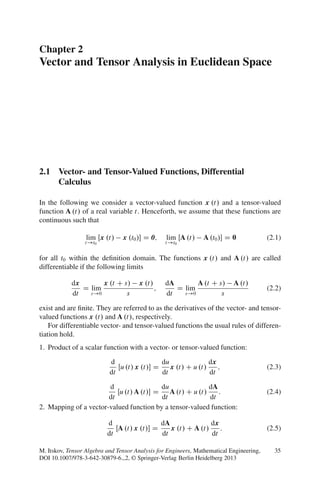
Example 2.1. Cylindrical coordinates in E3
. The cylindrical coordinates (Fig. 2.1)
are defined by
r D r .'; z; r/ D r cos 'e1 C r sin 'e2 C ze3 (2.17)
and
r D
q
.r e1/2
C .r e2/2
; z D r e3;
' D
8
<
:
arccos
r e1
r
if r e2 0;
2 arccos
r e1
r
if r e2 < 0;
(2.18)
where ei .i D 1; 2; 3/ form an orthonormal basis in E3
.
4. 38 2 Vector and Tensor Analysis in Euclidean Space
ϕ
e1
r
x1
e2 x2
x3
= z
e3
r
g3
g1
g2
Fig. 2.1 Cylindrical coordinates in three-dimensional space
The vector components with respect to a fixed basis, say H D fh1; h2; : : : ;
hng, obviously represent its coordinates. Indeed, according to Theorem 1.5 of the
previous chapter the following correspondence is one to one
r D xi
hi , xi
D r hi
; i D 1; 2; : : : ; n; (2.19)
where r 2 En
and H0
D
˚
h1
; h2
; : : : ; hn
«
is the basis dual to H. The components
xi
(2.19)2 are referred to as the linear coordinates of the vector r.
The Cartesian coordinates result as a special case of the linear coordinates (2.19)
where hi D ei .i D 1; 2; : : : ; n/ so that
r D xi
ei , xi
D r ei ; i D 1; 2; : : : ; n: (2.20)
Let xi
D xi
.r/ and yi
D yi
.r/ .i D 1; 2; : : : ; n/ be two arbitrary coordinate
systems in En
. Since their correspondences are one to one, the functions
xi
D Oxi
y1
; y2
; : : : ; yn
, yi
D Oyi
x1
; x2
; : : : ; xn
; i D 1; 2; : : : ; n (2.21)
are invertible. These functions describe the transformation of the coordinate sys-
tems. Inserting one relation (2.21) into another one yields
yi
D Oyi
Ox1
y1
; y2
; : : : ; yn
;
Ox2
y1
; y2
; : : : ; yn
; : : : ; Oxn
y1
; y2
; : : : ; yn
: (2.22)
5. 2.2 Coordinates in Euclidean Space, Tangent Vectors 39
The further differentiation with respect to yj
delivers with the aid of the chain rule
@yi
@yj
D ıij D
@yi
@xk
@xk
@yj
; i; j D 1; 2; : : : ; n: (2.23)
The determinant of the matrix (2.23) takes the form
ˇ
ˇıij
ˇ
ˇ D 1 D
ˇ
ˇ
ˇ
ˇ
@yi
@xk
@xk
@yj
ˇ
ˇ
ˇ
ˇ D
ˇ
ˇ
ˇ
ˇ
@yi
@xk
ˇ
ˇ
ˇ
ˇ
ˇ
ˇ
ˇ
ˇ
@xk
@yj
ˇ
ˇ
ˇ
ˇ : (2.24)
The determinant
ˇ
ˇ@yi
=@xk
ˇ
ˇ on the right hand side of (2.24) is referred to as Jacobian
determinant of the coordinate transformation yi
D Oyi
x1
; x2
; : : : ; xn
.i D 1; 2;
: : : ; n/. Thus, we have proved the following theorem.
Theorem 2.1. If the transformation of the coordinates yi
D Oyi
x1
; x2
; : : : ; xn
admits an inverse form xi
D Oxi
y1
; y2
; : : : ; yn
.i D 1; 2; : : : ; n/ and if J and K
are the Jacobians of these transformations then JK D 1.
One of the important consequences of this theorem is that
J D
ˇ
ˇ
ˇ
ˇ
@yi
@xk
ˇ
ˇ
ˇ
ˇ ¤ 0: (2.25)
Now, we consider an arbitrary curvilinear coordinate system
Âi
D Âi
.r/ , r D r Â1
; Â2
; : : : ; Ân
; (2.26)
where r 2 En
and Âi
2 R .i D 1; 2; : : : ; n/. The equations
Âi
D const; i D 1; 2; : : : ; k 1; k C 1; : : : ; n (2.27)
define a curve in En
called Âk
-coordinate line. The vectors (see Fig. 2.2)
gk D
@r
@Âk
; k D 1; 2; : : : ; n (2.28)
are called the tangent vectors to the corresponding Âk
-coordinate lines (2.27).
One can verify that the tangent vectors are linearly independent and form thus
a basis of En
. Conversely, let the vectors (2.28) be linearly dependent. Then, there
are scalars ˛i
2 R .i D 1; 2; : : : ; n/, not all zero, such that ˛i
gi D 0. Let further
xi
D xi
.r/ .i D 1; 2; : : : ; n/ be linear coordinates in En
with respect to a basis
H D fh1; h2; : : : ; hng. Then,
0 D ˛i
gi D ˛i @r
@Âi
D ˛i @r
@xj
@xj
@Âi
D ˛i @xj
@Âi
hj :
6. 40 2 Vector and Tensor Analysis in Euclidean Space
gk
r(θk + s)
r(θk)
θkΔr
Fig. 2.2 Illustration of the tangent vectors
Since the basis vectors hj .j D 1; 2; : : : ; n/ are linearly independent
˛i @xj
@Âi
D 0; j D 1; 2; : : : ; n:
This is a homogeneous linear equation system with a non-trivial solution
˛i
.i D 1; 2; : : : ; n/. Hence,
ˇ
ˇ@xj
=@Âi
ˇ
ˇ D 0, which obviously contradicts rela-
tion (2.25).
Example 2.2. Tangent vectors and metric coefficients of cylindrical coordinates
in E3
. By means of (2.17) and (2.28) we obtain
g1 D
@r
@'
D r sin 'e1 C r cos 'e2;
g2 D
@r
@z
D e3;
g3 D
@r
@r
D cos 'e1 C sin 'e2: (2.29)
The metric coefficients take by virtue of (1.24) and (1.25)2 the form
gij D gi gj D
2
4
r2
0 0
0 1 0
0 0 1
3
5 ; gij
D gij
1
D
2
4
r 2
0 0
0 1 0
0 0 1
3
5 : (2.30)
The dual basis results from (1.21)1 by
g1
D
1
r2
g1 D
1
r
sin 'e1 C
1
r
cos 'e2;
g2
D g2 D e3;
g3
D g3 D cos 'e1 C sin 'e2: (2.31)
7. 2.3 Co-, Contra- and Mixed Variant Components 41
2.3 Coordinate Transformation. Co-, Contra- and Mixed
Variant Components
Let Âi
D Âi
.r/ and NÂi
D NÂi
.r/ .i D 1; 2; : : : ; n/ be two arbitrary coordinate
systems in En
. It holds
Ngi D
@r
@ NÂi
D
@r
@Âj
@Âj
@ NÂi
D gj
@Âj
@ NÂi
; i D 1; 2; : : : ; n: (2.32)
If gi
is the dual basis to gi .i D 1; 2; : : : ; n/, then we can write
Ngi
D gj @ NÂi
@Âj
; i D 1; 2; : : : ; n: (2.33)
Indeed,
Ngi
Ngj D gk @ NÂi
@Âk
! Â
gl
@Âl
@ NÂj
Ã
D gk
gl
@ NÂi
@Âk
@Âl
@ NÂj
!
D ık
l
@ NÂi
@Âk
@Âl
@ NÂj
!
D
@ NÂi
@Âk
@Âk
@ NÂj
D
@ NÂi
@ NÂj
D ıi
j ; i; j D 1; 2; : : : ; n: (2.34)
One can observe the difference in the transformation of the dual vectors (2.32)
and (2.33) which results from the change of the coordinate system. The transforma-
tion rules of the form (2.32) and (2.33) and the corresponding variables are referred
to as covariant and contravariant, respectively. Covariant and contravariant variables
are denoted by lower and upper indices, respectively.
The co- and contravariant rules can also be recognized in the transformation
of the components of vectors and tensors if they are related to tangent vectors.
Indeed, let
x D xi gi
D xi
gi D Nxi Ngi
D Nxi
Ngi ; (2.35)
A D Aij gi
˝ gj
D Aij
gi ˝ gj D Ai
j gi ˝ gj
D NAij Ngi
˝ Ngj
D NA
ij
Ngi ˝ Ngj D NA
i
j Ngi ˝ Ngj
: (2.36)
Then, by means of (1.28), (1.88), (2.32) and (2.33) we obtain
Nxi D x Ngi D x
Â
gj
@Âj
@ NÂi
Ã
D xj
@Âj
@ NÂi
; (2.37)
Nxi
D x Ngi
D x gj @ NÂi
@Âj
!
D xj @ NÂi
@Âj
; (2.38)
8. 42 2 Vector and Tensor Analysis in Euclidean Space
NAij D Ngi A Ngj D
Â
gk
@Âk
@ NÂi
Ã
A
Â
gl
@Âl
@ NÂj
Ã
D
@Âk
@ NÂi
@Âl
@ NÂj
Akl ; (2.39)
NA
ij
D Ngi
A Ngj
D gk @ NÂi
@Âk
!
A gl @ NÂj
@Âl
!
D
@ NÂi
@Âk
@ NÂj
@Âl
Akl
; (2.40)
NA
i
j D Ngi
A Ngj D gk @ NÂi
@Âk
!
A
Â
gl
@Âl
@ NÂj
Ã
D
@ NÂi
@Âk
@Âl
@ NÂj
Ak
l : (2.41)
Accordingly, the vector and tensor components xi , Aij and xi
, Aij
are called
covariant and contravariant, respectively. The tensor components Ai
j are referred
to as mixed variant. The transformation rules (2.37)–(2.41) can similarly be written
for tensors of higher orders as well. For example, one obtains for third-order tensors
NAijk D
@Âr
@ NÂi
@Âs
@ NÂj
@Ât
@ NÂk
Arst ; NAijk
D
@ NÂi
@Âr
@ NÂj
@Âs
@ NÂk
@Ât
Arst
; : : : (2.42)
From the very beginning we have supplied coordinates with upper indices which
imply the contravariant transformation rule. Indeed, let us consider the transforma-
tion of a coordinate system NÂi
D NÂi
Â1
; Â2
; : : : ; Ân
.i D 1; 2; : : : ; n/. It holds:
d NÂi
D
@ NÂi
@Âk
dÂk
; i D 1; 2; : : : ; n: (2.43)
Thus, the differentials of the coordinates really transform according to the con-
travariant law (2.33).
Example 2.3. Transformation of linear coordinates into cylindrical ones (2.17).
Let xi
D xi
.r/ be linear coordinates with respect to an orthonormal basis
ei .i D 1; 2; 3/ in E3
:
xi
D r ei , r D xi
ei : (2.44)
By means of (2.17) one can write
x1
D r cos '; x2
D r sin '; x3
D z (2.45)
and consequently
@x1
@'
D r sin ' D x2
;
@x1
@z
D 0;
@x1
@r
D cos ' D
x1
r
;
@x2
@'
D r cos ' D x1
;
@x2
@z
D 0;
@x2
@r
D sin ' D
x2
r
;
@x3
@'
D 0;
@x3
@z
D 1;
@x3
@r
D 0:
(2.46)
9. 2.4 Gradient, Covariant and Contravariant Derivatives 43
The reciprocal derivatives can easily be obtained from (2.23) by inverting the matrixh
@xi
@'
@xi
@z
@xi
@r
i
. This yields:
@'
@x1
D
1
r
sin ' D
x2
r2
;
@'
@x2
D
1
r
cos ' D
x1
r2
;
@'
@x3
D 0;
@z
@x1
D 0;
@z
@x2
D 0;
@z
@x3
D 1;
@r
@x1
D cos ' D
x1
r
;
@r
@x2
D sin ' D
x2
r
;
@r
@x3
D 0:
(2.47)
2.4 Gradient, Covariant and Contravariant Derivatives
Let ˚ D ˚ Â1
; Â2
; : : : ; Ân
, x D x Â1
; Â2
; : : : ; Ân
and A D A Â1
; Â2
; : : : ; Ân
be, respectively, a scalar-, a vector- and a tensor-valued differentiable function of the
coordinates Âi
2 R .i D 1; 2; : : : ; n/. Such functions of coordinates are generally
referred to as fields, as for example, the scalar field, the vector field or the tensor
field. Due to the one to one correspondence (2.26) these fields can alternatively be
represented by
˚ D ˚ .r/ ; x D x .r/ ; A D A .r/ : (2.48)
In the following we assume that the so-called directional derivatives of the func-
tions (2.48)
d
ds
˚ .r C sa/
ˇ
ˇ
ˇ
ˇ
sD0
D lim
s!0
˚ .r C sa/ ˚ .r/
s
;
d
ds
x .r C sa/
ˇ
ˇ
ˇ
ˇ
sD0
D lim
s!0
x .r C sa/ x .r/
s
;
d
ds
A .r C sa/
ˇ
ˇ
ˇ
ˇ
sD0
D lim
s!0
A .r C sa/ A .r/
s
(2.49)
exist for all a 2 En
. Further, one can show that the mappings a ! d
ds ˚ .r C sa/
ˇ
ˇ
sD0
,
a ! d
ds
x .r C sa/
ˇ
ˇ
sD0
and a ! d
ds
A .r C sa/
ˇ
ˇ
sD0
are linear with respect to the
vector a. For example, we can write for the directional derivative of the scalar
function ˚ D ˚ .r/
d
ds
˚ Œr C s .a C b/
ˇ
ˇ
ˇ
ˇ
sD0
D
d
ds
˚ Œr C s1a C s2b
ˇ
ˇ
ˇ
ˇ
sD0
; (2.50)
10. 44 2 Vector and Tensor Analysis in Euclidean Space
where s1 and s2 are assumed to be functions of s such that s1 D s and s2 D s. With
the aid of the chain rule this delivers
d
ds
˚ Œr C s1a C s2b
ˇ
ˇ
ˇ
ˇ
sD0
D
@
@s1
˚ Œr C s1a C s2b
ds1
ds
C
@
@s2
˚ Œr C s1a C s2b
ds2
ds
ˇ
ˇ
ˇ
ˇ
sD0
D
@
@s1
˚ .r C s1a C s2b/
ˇ
ˇ
ˇ
ˇ
s1D0;s2D0
C
@
@s2
˚ .r C s1a C s2b/
ˇ
ˇ
ˇ
ˇ
s1D0;s2D0
D
d
ds
˚ .r C sa/
ˇ
ˇ
ˇ
ˇ
sD0
C
d
ds
˚ .r C sb/
ˇ
ˇ
ˇ
ˇ
sD0
and finally
d
ds
˚ Œr C s .a C b/
ˇ
ˇ
ˇ
ˇ
sD0
D
d
ds
˚ .r C sa/
ˇ
ˇ
ˇ
ˇ
sD0
C
d
ds
˚ .r C sb/
ˇ
ˇ
ˇ
ˇ
sD0
(2.51)
for all a; b 2 En
. In a similar fashion we can write
d
ds
˚ .r C s˛a/
ˇ
ˇ
ˇ
ˇ
sD0
D
d
d .˛s/
˚ .r C s˛a/
d .˛s/
ds
ˇ
ˇ
ˇ
ˇ
sD0
D ˛
d
ds
˚ .r C sa/
ˇ
ˇ
ˇ
ˇ
sD0
; 8a 2 En
; 8˛ 2 R: (2.52)
Representing a with respect to a basis as a D ai
gi we thus obtain
d
ds
˚ .r C sa/
ˇ
ˇ
ˇ
ˇ
sD0
D
d
ds
˚ r C sai
gi
ˇ
ˇ
ˇ
ˇ
sD0
D ai d
ds
˚ .r C sgi /
ˇ
ˇ
ˇ
ˇ
sD0
D
d
ds
˚ .r C sgi /
ˇ
ˇ
ˇ
ˇ
sD0
gi
aj
gj ; (2.53)
where gi
form the basis dual to gi .i D 1; 2; : : : ; n/. This result can finally be
expressed by
d
ds
˚ .r C sa/
ˇ
ˇ
ˇ
ˇ
sD0
D grad˚ a; 8a 2 En
; (2.54)
where the vector denoted by grad˚ 2 En
is referred to as gradient of the function
˚ D ˚ .r/. According to (2.53) and (2.54) it can be represented by
grad˚ D
d
ds
˚ .r C sgi /
ˇ
ˇ
ˇ
ˇ
sD0
gi
: (2.55)
11. 2.4 Gradient, Covariant and Contravariant Derivatives 45
Example 2.4. Gradient of the scalar function krk. Using the definition of the
directional derivative (2.49) we can write
d
ds
kr C sak
ˇ
ˇ
ˇ
ˇ
sD0
D
d
ds
p
.r C sa/ .r C sa/
ˇ
ˇ
ˇ
ˇ
sD0
D
d
ds
p
r r C 2s .r a/ C s2 .a a/
ˇ
ˇ
ˇ
ˇ
sD0
D
1
2
2 .r a/ C 2s .a a/
p
r r C 2s .r a/ C s2 .a a/
ˇ
ˇ
ˇ
ˇ
ˇ
sD0
D
r a
krk
:
Comparing this result with (2.54) delivers
grad krk D
r
krk
: (2.56)
Similarly to (2.54) one defines the gradient of the vector function x D x .r/ and the
gradient of the tensor function A D A .r/:
d
ds
x .r C sa/
ˇ
ˇ
ˇ
ˇ
sD0
D .gradx/ a; 8a 2 En
; (2.57)
d
ds
A .r C sa/
ˇ
ˇ
ˇ
ˇ
sD0
D .gradA/ a; 8a 2 En
: (2.58)
Herein, gradx and gradA represent tensors of second and third order, respectively.
In order to evaluate the above gradients (2.54), (2.57) and (2.58) we represent the
vectors r and a with respect to the linear coordinates (2.19) as
r D xi
hi ; a D ai
hi : (2.59)
With the aid of the chain rule we can further write for the directional derivative of
the function ˚ D ˚ .r/:
d
ds
˚ .r C sa/
ˇ
ˇ
ˇ
ˇ
sD0
D
d
ds
˚ xi
C sai
hi
ˇ
ˇ
ˇ
ˇ
sD0
D
@˚
@ .xi C sai /
d xi
C sai
ds
ˇ
ˇ
ˇ
ˇ
ˇ
sD0
D
@˚
@xi
ai
D
Â
@˚
@xi
hi
Ã
aj
hj D
Â
@˚
@xi
hi
Ã
a; 8a 2 En
:
12. 46 2 Vector and Tensor Analysis in Euclidean Space
Comparing this result with (2.54) and bearing in mind that it holds for all vectors a
we obtain
grad˚ D
@˚
@xi
hi
: (2.60)
The representation (2.60) can be rewritten in terms of arbitrary curvilinear coordi-
nates r D r Â1
; Â2
; : : : ; Ân
and the corresponding tangent vectors (2.28). Indeed,
in view of (2.33) and (2.60)
grad˚ D
@˚
@xi
hi
D
@˚
@Âk
@Âk
@xi
hi
D
@˚
@Âi
gi
: (2.61)
Comparison of the last result with (2.55) yields
d
ds
˚ .r C sgi /
ˇ
ˇ
ˇ
ˇ
sD0
D
@˚
@Âi
; i D 1; 2; : : : ; n: (2.62)
According to the definition (2.54) the gradient is independent of the choice
of the coordinate system. This can also be seen from relation (2.61). Indeed,
taking (2.33) into account we can write for an arbitrary coordinate system NÂi
D
NÂi
Â1
; Â2
; : : : ; Ân
.i D 1; 2; : : : ; n/:
grad˚ D
@˚
@Âi
gi
D
@˚
@ NÂj
@ NÂj
@Âi
gi
D
@˚
@ NÂj
Ngj
: (2.63)
Similarly to relation (2.61) one can express the gradients of the vector-valued
function x D x .r/ and the tensor-valued function A D A .r/ by
gradx D
@x
@Âi
˝ gi
; gradA D
@A
@Âi
˝ gi
: (2.64)
Example 2.5. Deformation gradient and its representation in the case of simple
shear. Let x and X be the position vectors of a material point in the current and
reference configuration, respectively. The deformation gradient F 2 Lin3
is defined
as the gradient of the function x .X/ as
F D gradx: (2.65)
For the Cartesian coordinates in E3
where x D xi
ei and X D Xi
ei we can write
by using (2.64)1
F D
@x
@Xj
˝ ej
D
@xi
@Xj
ei ˝ ej
D Fi
j ei ˝ ej
; (2.66)
13. 2.4 Gradient, Covariant and Contravariant Derivatives 47
X2
X
X2
, x2
X1
, x 1
X1
X1
x
ϕ
e2
e1
γX2
Fig. 2.3 Simple shear of a rectangular sheet
where the matrix
h
Fi
j
i
is given by
h
Fi
j
i
D
2
6
6
6
6
6
4
@x1
@X1
@x1
@X2
@x1
@X3
@x2
@X1
@x2
@X2
@x2
@X3
@x3
@X1
@x3
@X2
@x3
@X3
3
7
7
7
7
7
5
: (2.67)
In the case of simple shear it holds (see Fig. 2.3)
x1
D X1
C X2
; x2
D X2
; x3
D X3
; (2.68)
where denotes the amount of shear. Insertion into (2.67) yields
h
Fi
j
i
D
2
4
1 0
0 1 0
0 0 1
3
5 : (2.69)
Henceforth, the derivatives of the functions ˚ D ˚ Â1
; Â2
; : : : ; Ân
, x D
x Â1
; Â2
; : : : ; Ân
and A D A Â1
; Â2
; : : : ; Ân
with respect to curvilinear coordi-
nates Âi
will be denoted shortly by
˚;i D
@˚
@Âi
; x;i D
@x
@Âi
; A;i D
@A
@Âi
: (2.70)
They obey the covariant transformation rule (2.32) with respect to the index i since
@˚
@Âi
D
@˚
@ NÂk
@ NÂk
@Âi
;
@x
@Âi
D
@x
@ NÂk
@ NÂk
@Âi
;
@A
@Âi
D
@A
@ NÂk
@ NÂk
@Âi
(2.71)
14. 48 2 Vector and Tensor Analysis in Euclidean Space
and represent again a scalar, a vector and a second-order tensor, respectively. The
latter ones can be represented with respect to a basis as
x;i D xj
ji gj D xj ji gj
;
A;i D Akl
ji gk ˝ gl D Aklji gk
˝ gl
D Ak
l ji gk ˝ gl
; (2.72)
where . /ji denotes some differential operator on the components of the vector x
or the tensor A. In view of (2.71) and (2.72) this operator transforms with respect
to the index i according to the covariant rule and is called covariant derivative. The
covariant type of the derivative is accentuated by the lower position of the coordinate
index.
On the basis of the covariant derivative we can also define the contravariant one.
To this end, we formally apply the rule of component transformation (1.95)1 as
. /ji
D gij
. /jj . Accordingly,
xj
ji
D gik
xj
jk; xj ji
D gik
xj jk;
Akl
ji
D gim
Akl
jm; Akl ji
D gim
Akljm; Ak
l ji
D gim
Ak
l jm : (2.73)
For scalar functions the covariant and the contravariant derivative are defined to be
equal to the partial one so that:
˚ji D ˚ji
D ˚;i : (2.74)
In view of (2.63)–(2.70), (2.72) and (2.74) the gradients of the functions ˚ D
˚ Â1
; Â2
; : : : ; Ân
, x D x Â1
; Â2
; : : : ; Ân
and A D A Â1
; Â2
; : : : ; Ân
take the
form
grad˚ D ˚ji gi
D ˚ji
gi ;
gradx D xj
ji gj ˝ gi
D xj ji gj
˝ gi
D xj
ji
gj ˝ gi D xj ji
gj
˝ gi ;
gradA D Akl
ji gk ˝ gl ˝ gi
D Aklji gk
˝ gl
˝ gi
D Ak
l ji gk ˝ gl
˝ gi
D Akl
ji
gk ˝ gl ˝ gi D Aklji
gk
˝ gl
˝ gi D Ak
l ji
gk ˝ gl
˝ gi :
(2.75)
2.5 Christoffel Symbols, Representation of the Covariant
Derivative
In the previous section we have introduced the notion of the covariant derivative but
have not so far discussed how it can be taken. Now, we are going to formulate a
procedure constructing the differential operator of the covariant derivative. In other
15. 2.5 Christoffel Symbols, Representation of the Covariant Derivative 49
words, we would like to express the covariant derivative in terms of the vector or
tensor components. To this end, the partial derivatives of the tangent vectors (2.28)
with respect to the coordinates are first needed. Since these derivatives again
represent vectors in En
, they can be expressed in terms of the tangent vectors gi
or dual vectors gi
.i D 1; 2; : : : ; n/ both forming bases of En
. Thus, one can write
gi ;j D €ijkgk
D €k
ij gk; i; j D 1; 2; : : : ; n; (2.76)
where the components €ijk and €k
ij .i; j; k D 1; 2; : : : ; n/ are referred to as the
Christoffel symbols of the first and second kind, respectively. In view of the
relation gk
D gkl
gl .k D 1; 2; : : : ; n/ (1.21) these symbols are connected with
each other by
€k
ij D gkl
€ijl ; i; j; k D 1; 2; : : : ; n: (2.77)
Keeping the definition of tangent vectors (2.28) in mind we further obtain
gi ;j D r;ij D r;ji D gj ;i ; i; j D 1; 2; : : : ; n: (2.78)
With the aid of (1.28) the Christoffel symbols can thus be expressed by
€ijk D €jik D gi ;j gk D gj ;i gk; (2.79)
€k
ij D €k
ji D gi ;j gk
D gj ;i gk
; i; j; k D 1; 2; : : : ; n: (2.80)
For the dual basis gi
.i D 1; 2; : : : ; n/ one further gets by differentiating the
identities gi
gj D ıi
j (1.15):
0 D ıi
j
Á
;k D gi
gj ;k D gi
;k gj C gi
gj ;k
D gi
;k gj C gi
€l
jkgl
Á
D gi
;k gj C €i
jk; i; j; k D 1; 2; : : : ; n:
Hence,
€i
jk D €i
kj D gi
;k gj D gi
;j gk; i; j; k D 1; 2; : : : ; n (2.81)
and consequently
gi
;k D €i
jkgj
D €i
kj gj
; i; k D 1; 2; : : : ; n: (2.82)
By means of the identities following from (2.79)
gij ;k D gi gj ;k D gi ;k gj C gi gj ;k D €ikj C €jki ; (2.83)
where i; j; k D 1; 2; : : : ; n and in view of (2.77) we finally obtain
16. 50 2 Vector and Tensor Analysis in Euclidean Space
€ijk D
1
2
gki ;j C gkj ;i gij ;k ; (2.84)
€k
ij D
1
2
gkl
gli ;j Cglj ;i gij ;l ; i; j; k D 1; 2; : : : ; n: (2.85)
It is seen from (2.84) and (2.85) that all Christoffel symbols identically vanish in the
Cartesian coordinates (2.20). Indeed, in this case
gij D ei ej D ıij ; i; j D 1; 2; : : : ; n (2.86)
and hence
€ijk D €k
ij D 0; i; j; k D 1; 2; : : : ; n: (2.87)
Example 2.6. Christoffel symbols for cylindrical coordinates in E3
(2.17). By
virtue of relation (2.30)1 we realize that g11;3 D 2r, while all other derivatives
gik;j .i; j; k D 1; 2; 3/ (2.83) are zero. Thus, Eq. (2.84) delivers
€131 D €311 D r; €113 D r; (2.88)
while all other Christoffel symbols of the first kind €ijk .i; j; k D 1; 2; 3/ are
likewise zero. With the aid of (2.77) and (2.30)2 we further obtain
€1
ij D g11
€ij1 D r 2
€ij1; €2
ij D g22
€ij 2 D €ij 2;
€3
ij D g33
€ij 3 D €ij 3; i; j D 1; 2; 3: (2.89)
By virtue of (2.88) we can further write
€1
13 D €1
31 D
1
r
; €3
11 D r; (2.90)
while all remaining Christoffel symbols of the second kind €k
ij .i; j; k D 1; 2; 3/
(2.85) vanish.
Now, we are in a position to express the covariant derivative in terms of the vector
or tensor components by means of the Christoffel symbols. For the vector-valued
function x D x Â1
; Â2
; : : : ; Ân
we can write using (2.76)
x;j D xi
gi ;j D xi
;j gi C xi
gi ;j
D xi
;j gi C xi
€k
ij gk D xi
;j Cxk
€i
kj
Á
gi ; (2.91)
or alternatively using (2.82)
17. 2.5 Christoffel Symbols, Representation of the Covariant Derivative 51
x;j D xi gi
;j D xi ;j gi
C xi gi
;j
D xi ;j gi
xi €i
kj gk
D xi ;j xk€k
ij
Á
gi
: (2.92)
Comparing these results with (2.72) yields
xi
jj D xi
;j Cxk
€i
kj ; xi jj D xi ;j xk€k
ij ; i; j D 1; 2; : : : ; n: (2.93)
Similarly, we treat the tensor-valued function A D A Â1
; Â2
; : : : ; Ân
:
A;k D Aij
gi ˝ gj ;k
D Aij
;k gi ˝ gj C Aij
gi ;k ˝gj C Aij
gi ˝ gj ;k
D Aij
;k gi ˝ gj C Aij
€l
ikgl ˝ gj C Aij
gi ˝ €l
jkgl
Á
D Aij
;k CAlj
€i
lk C Ail
€
j
lk
Á
gi ˝ gj : (2.94)
Thus,
Aij
jkD Aij
;k CAlj
€i
lk C Ail
€
j
lk; i; j; k D 1; 2; : : : ; n: (2.95)
By analogy, we further obtain
Aij jkD Aij ;k Alj €l
ik Ail €l
jk;
Ai
j jkD Ai
j ;k CAl
j €i
lk Ai
l €l
jk; i; j; k D 1; 2; : : : ; n: (2.96)
Similar expressions for the covariant derivative can also be formulated for tensors
of higher orders.
From (2.87), (2.93), (2.95) and (2.96) it is seen that the covariant derivative taken
in Cartesian coordinates (2.20) coincides with the partial derivative:
xi
jj D xi
;j ; xi jj D xi ;j ;
Aij
jkD Aij
;k ; Aij jkD Aij ;k ; Ai
j jkD Ai
j ;k ; i; j; k D 1; 2; : : : ; n: (2.97)
Formal application of the covariant derivative (2.93), (2.95) and (2.96) to
the tangent vectors (2.28) and metric coefficients (1.90)1;2 yields by virtue
of (2.76), (2.77), (2.82) and (2.84) the following identities referred to as Ricci’s
Theorem:
gi jj D gi ;j gl €l
ij D 0; gi
jj D gi
;j Cgl
€i
lj D 0; (2.98)
18. 52 2 Vector and Tensor Analysis in Euclidean Space
gij jkD gij ;k glj €l
ik gil €l
jk D gij ;k €ikj €jki D 0; (2.99)
gij
jkD gij
;k Cglj
€i
lk C gil
€
j
lk D gil
gjm
. glm;k C€mkl C €lkm/ D 0; (2.100)
where i; j; k D 1; 2; : : : ; n. The latter two identities can alternatively be proved
by taking (1.25) into account and using the product rules of differentiation for the
covariant derivative which can be written as (Exercise 2.7)
Aij jkD ai jk bj C ai bj jk for Aij D ai bj ; (2.101)
Aij
jkD ai
jk bj
C ai
bj
jk for Aij
D ai
bj
; (2.102)
Ai
j jk D ai
jk bj C ai
bj jk for Ai
j D ai
bj ; i; j; k D 1; 2; : : : ; n: (2.103)
2.6 Applications in Three-Dimensional Space:
Divergence and Curl
Divergence of a tensor field. One defines the divergence of a tensor field S .r/ by
divS D lim
V !0
1
V
Z
A
SndA; (2.104)
where the integration is carried out over a closed surface area A with the volume V
and the outer unit normal vector n illustrated in Fig. 2.4.
For the integration we consider a curvilinear parallelepiped with the edges
formed by the coordinate lines Â1
; Â2
; Â3
and Â1
C Â1
; Â2
C Â2
; Â3
C Â3
(Fig. 2.5). The infinitesimal surface elements of the parallelepiped can be defined
in a vector form by
dA.i/
D ˙ dÂj
gj dÂk
gk D ˙ggi
dÂj
dÂk
; i D 1; 2; 3; (2.105)
where g D Œg1g2g3 (1.31) and i; j; k is an even permutation of 1,2,3. The corre-
sponding infinitesimal volume element can thus be given by (no summation over
i)
dV D dA.i/
dÂi
gi D dÂ1
g1 dÂ2
g2 dÂ3
g3
D Œg1g2g3 dÂ1
dÂ2
dÂ3
D gdÂ1
dÂ2
dÂ3
: (2.106)
We also need the identities
19. 2.6 Applications in Three-Dimensional Space: Divergence and Curl 53
dA
n
V
Fig. 2.4 Definition of the divergence: closed surface with the area A, volume V and the outer unit
normal vector n
Fig. 2.5 Derivation of the divergence in three-dimensional space
g;k D Œg1g2g3 ;k D €l
1k Œgl g2g3 C €l
2k Œg1gl g3 C €l
3k Œg1g2gl
D €l
lk Œg1g2g3 D €l
lkg; (2.107)
ggi
;i D g;i gi
C ggi
;i D €l
li ggi
€i
li ggl
D 0; (2.108)
following from (1.39), (2.76) and (2.82). With these results in hand, one can express
the divergence (2.104) as follows
divS D lim
V !0
1
V
Z
A
SndA
D lim
V !0
1
V
3X
iD1
Z
A.i/
h
S Âi
C Âi
dA.i/
Âi
C Âi
C S Âi
dA.i/
Âi
i
:
Keeping (2.105) and (2.106) in mind and using the abbreviation
20. 54 2 Vector and Tensor Analysis in Euclidean Space
si
Âi
D S Âi
g Âi
gi
Âi
; i D 1; 2; 3 (2.109)
we can thus write
divS D lim
V !0
1
V
3X
iD1
ÂkCÂk
Z
Âk
Âj CÂj
Z
Âj
si
Âi
C Âi
si
Âi
dÂj
dÂk
D lim
V !0
1
V
3X
iD1
ÂkCÂk
Z
Âk
Âj CÂj
Z
Âj
Âi CÂi
Z
Âi
@si
@Âi
dÂi
dÂj
dÂk
D lim
V !0
1
V
3X
iD1
Z
V
si
;i
g
dV; (2.110)
where i; j; k is again an even permutation of 1,2,3. Assuming continuity of the
integrand in (2.110) and applying (2.108) and (2.109) we obtain
divS D
1
g
si
;i D
1
g
Sggi
;i D
1
g
S;i ggi
C S ggi
;i D S;i gi
; (2.111)
which finally yields by virtue of (2.72)2
divS D S;i gi
D S i
j ji gj
D Sji
ji gj : (2.112)
Example 2.7. The momentum balance in Cartesian and cylindrical coordinates. Let
us consider a material body or a part of it with a mass m, volume V and outer surface
A. According to the Euler law of motion the vector sum of external volume forces
f dV and surface tractions tdA results in the vector sum of inertia forces Rxdm,
where x stands for the position vector of a material element dm and the superposed
dot denotes the material time derivative. Hence,
Z
m
Rxdm D
Z
A
tdA C
Z
V
f dV: (2.113)
Applying the Cauchy theorem (1.77) to the first integral on the right hand side and
using the identity dm D dV it further delivers
Z
V
RxdV D
Z
A
ndA C
Z
V
f dV; (2.114)
where denotes the density of the material. Dividing this equation by V and
considering the limit case V ! 0 we obtain by virtue of (2.104)
21. 2.6 Applications in Three-Dimensional Space: Divergence and Curl 55
Rx D div C f : (2.115)
This vector equation is referred to as the momentum balance.
Representing vector and tensor variables with respect to the tangent vectors
gi .i D 1; 2; 3/ of an arbitrary curvilinear coordinate system as
Rx D ai
gi ; D ij
gi ˝ gj ; f D f i
gi
and expressing the divergence of the Cauchy stress tensor by (2.112) we obtain the
component form of the momentum balance (2.115) by
ai
D ij
jj Cf i
; i D 1; 2; 3: (2.116)
With the aid of (2.95) the covariant derivative of the Cauchy stress tensor can further
be written by
ij
jkD ij
;k C lj
€i
lk C il
€
j
lk; i; j; k D 1; 2; 3 (2.117)
and thus,
ij
jj D ij
;j C lj
€i
lj C il
€
j
lj ; i D 1; 2; 3: (2.118)
By virtue of the expressions for the Christoffel symbols (2.90) and keeping in mind
the symmetry of the Cauchy stress tensors ij
D ji
.i ¤ j D 1; 2; 3/ we thus
obtain for cylindrical coordinates:
1j
jj D 11
;' C 12
;z C 13
;r C
3 31
r
;
2j
jj D 21
;' C 22
;z C 23
;r C
32
r
;
3j
jj D 31
;' C 32
;z C 33
;r r 11
C
33
r
: (2.119)
The balance equations finally take the form
a1
D 11
;' C 12
;z C 13
;r C
3 31
r
C f 1
;
a2
D 21
;' C 22
;z C 23
;r C
32
r
C f 2
;
a3
D 31
;' C 32
;z C 33
;r r 11
C
33
r
C f 3
: (2.120)
In Cartesian coordinates, where gi D ei .i D 1; 2; 3/, the covariant derivative
coincides with the partial one, so that
22. 56 2 Vector and Tensor Analysis in Euclidean Space
ij
jj D ij
;j D ij ;j : (2.121)
Thus, the balance equations reduce to
Rx1 D 11;1 C 12;2 C 13;3 Cf1;
Rx2 D 21;1 C 22;2 C 23;3 Cf2;
Rx3 D 31;1 C 32;2 C 33;3 Cf3; (2.122)
where Rxi D ai .i D 1; 2; 3/.
Divergence and curl of a vector field. Now, we consider a differentiable vector
field t Â1
; Â2
; Â3
. One defines the divergence and curl of t Â1
; Â2
; Â3
respec-
tively by
divt D lim
V !0
1
V
Z
A
.t n/ dA; (2.123)
curlt D lim
V !0
1
V
Z
A
.n t/ dA D lim
V !0
1
V
Z
A
.t n/ dA; (2.124)
where the integration is again carried out over a closed surface area A with the
volume V and the outer unit normal vector n (see Fig. 2.4). Considering (1.66)
and (2.104), the curl can also be represented by
curlt D lim
V !0
1
V
Z
A
OtndA D divOt: (2.125)
Treating the vector field in the same manner as the tensor field we can write
divt D t;i gi
D ti
ji (2.126)
and in view of (2.75)2 (see also Exercise 1.44)
divt D tr .gradt/ : (2.127)
The same procedure applied to the curl (2.124) leads to
curlt D gi
t;i : (2.128)
By virtue of (2.72)1 and (1.44) we further obtain (see also Exercise 2.8)
curlt D ti jj gj
gi
D ejik 1
g
ti jj gk: (2.129)
With respect to the Cartesian coordinates (2.20) with gi D ei .i D 1; 2; 3/ the
divergence (2.126) and curl (2.129) simplify to
23. 2.6 Applications in Three-Dimensional Space: Divergence and Curl 57
divt D ti
;i D t1
;1 Ct2
;2 Ct3
;3 D t1;1 Ct2;2 Ct3;3 ; (2.130)
curlt D ejik
ti ;j ek
D .t3;2 t2;3 / e1 C .t1;3 t3;1 / e2 C .t2;1 t1;2 / e3: (2.131)
Now, we are going to discuss some combined operations with a gradient, divergence,
curl, tensor mapping and products of various types (see also Exercise 2.12).
1. Curl of a gradient:
curl grad˚ D 0: (2.132)
2. Divergence of a curl:
div curlt D 0: (2.133)
3. Divergence of a vector product:
div .u v/ D v curlu u curlv: (2.134)
4. Gradient of a divergence:
grad divt D div .gradt/T
; (2.135)
grad divt D curl curlt C div gradt D curl curlt C t; (2.136)
where the combined operator t D div gradt is known as the Laplacian.
5. Skew-symmetric part of a gradient
skew .gradt/ D
1
2
dcurlt: (2.137)
6. Divergence of a (left) mapping
div .tA/ D A W gradt C t divA: (2.138)
7. Divergence of a product of a scalar-valued function and a vector-valued function
div .˚t/ D t grad˚ C ˚divt: (2.139)
8. Divergence of a product of a scalar-valued function and a tensor-valued function
div .˚A/ D Agrad˚ C ˚divA: (2.140)
We prove, for example, identity (2.132). To this end, we apply (2.75)1, (2.82)
and (2.128). Thus, we write
24. 58 2 Vector and Tensor Analysis in Euclidean Space
curl grad˚ D gj
˚ji gi
;j D ˚;ij gj
gi
C ˚;i gj
gi
;j
D ˚;ij gj
gi
˚;i €i
kj gj
gk
D 0 (2.141)
taking into account that ˚;ij D ˚;ji , €l
ij D €l
ji and gi
gj
D gj
gi
.i ¤ j; i; j D 1; 2; 3/.
Example 2.8. Balance of mechanical energy as an integral form of the momentum
balance. Using the above identities we are now able to formulate the balance of
mechanical energy on the basis of the momentum balance (2.115). To this end, we
multiply this vector relation scalarly by the velocity vector v D Px
v . Rx/ D v div C v f :
Using (2.138) we can further write
v . Rx/ C W gradv D div .v / C v f :
Integrating this relation over the volume of the body V yields
d
dt
Z
m
Â
1
2
v v
Ã
dm C
Z
V
W gradvdV D
Z
V
div .v / dV C
Z
V
v f dV;
where again dm D dV and m denotes the mass of the body. Keeping in mind
the definition of the divergence (2.104) and applying the Cauchy theorem (1.77)
according to which the Cauchy stress vector is given by t D n, we finally obtain
the relation
d
dt
Z
m
Â
1
2
v v
Ã
dm C
Z
V
W gradvdV D
Z
A
v tdA C
Z
V
v f dV (2.142)
expressing the balance of mechanical energy. Indeed, the first and the second
integrals on the left hand side of (2.142) represent the time rate of the kinetic energy
and the stress power, respectively. The right hand side of (2.142) expresses the power
of external forces i.e. external tractions t on the boundary of the body A and external
volume forces f inside of it.
Example 2.9. Axial vector of the spin tensor. The spin tensor is defined as a skew-
symmetric part of the velocity gradient by
w D skew .gradv/ : (2.143)
By virtue of (1.158) we can represent it in terms of the axial vector
25. 2.6 Applications in Three-Dimensional Space: Divergence and Curl 59
w D Ow; (2.144)
which in view of (2.137) takes the form:
w D
1
2
curlv: (2.145)
Example 2.10. Navier-Stokes equations for a linear-viscous fluid in Cartesian and
cylindrical coordinates. A linear-viscous fluid (also called Newton fluid or Navier-
Poisson fluid) is defined by a constitutive equation
D pI C 2Ád C .trd/ I; (2.146)
where
d D sym .gradv/ D
1
2
gradv C .gradv/T
(2.147)
denotes the rate of deformation tensor, p is the hydrostatic pressure while Á and
represent material constants referred to as shear viscosity and second viscosity
coefficient, respectively. Inserting (2.147) into (2.146) and taking (2.127) into
account delivers
D pI C Á gradv C .gradv/T
C .divv/ I: (2.148)
Substituting this expression into the momentum balance (2.115) and using (2.135)
and (2.140) we obtain the relation
Pv D gradp C Ádiv gradv C .Á C / grad divv C f (2.149)
referred to as the Navier-Stokes equation. By means of (2.136) it can be rewritten as
Pv D gradp C .2Á C / grad divv Ácurl curlv C f : (2.150)
For an incompressible fluid characterized by the kinematic condition trd D divv D
0, the latter two equations simplify to
Pv D gradp C Áv C f ; (2.151)
Pv D gradp Ácurl curlv C f : (2.152)
With the aid of the identity v D v;iji
(see Exercise 2.14) we thus can write
Pv D gradp C Áv;iji
Cf : (2.153)
26. 60 2 Vector and Tensor Analysis in Euclidean Space
In Cartesian coordinates this relation is thus written out as
Pvi D p;i CÁ .vi ;11 Cvi ;22 Cvi ;33 / C fi ; i D 1; 2; 3: (2.154)
For arbitrary curvilinear coordinates we use the following representation for the
vector Laplacian (see Exercise 2.16)
v D gij
vk
;ij C2€k
li vl
;j €m
ij vk
;m C€k
li ;j vl
C €k
mj €m
li vl
€m
ij €k
lmvl
Á
gk:
(2.155)
For the cylindrical coordinates it takes by virtue of (2.30) and (2.90) the following
form
v D r 2
v1
;11 Cv1
;22 Cv1
;33 C3r 1
v1
;3 C2r 3
v3
;1 g1
C r 2
v2
;11 Cv2
;22 Cv2
;33 Cr 1
v2
;3 g2
C r 2
v3
;11 Cv3
;22 Cv3
;33 2r 1
v1
;1 Cr 1
v3
;3 r 2
v3
g3:
Inserting this result into (2.151) and using the representations Pv D Pvi
gi and f D
f i
gi we finally obtain
Pv1
D f 1 @p
@'
C Á
Â
1
r2
@2
v1
@'2
C
@2
v1
@z2
C
@2
v1
@r2
C
3
r
@v1
@r
C
2
r3
@v3
@'
Ã
;
Pv2
D f 2 @p
@z
C Á
Â
1
r2
@2
v2
@'2
C
@2
v2
@z2
C
@2
v2
@r2
C
1
r
@v2
@r
Ã
;
Pv3
D f 3 @p
@r
C Á
Â
1
r2
@2
v3
@'2
C
@2
v3
@z2
C
@2
v3
@r2
2
r
@v1
@'
C
1
r
@v3
@r
v3
r2
Ã
: (2.156)
Exercises
2.1. Evaluate tangent vectors, metric coefficients and the dual basis of spherical
coordinates in E3
defined by (Fig. 2.6)
r .'; ; r/ D r sin ' sin e1 C r cos e2 C r cos ' sin e3: (2.157)
2.2. Evaluate the coefficients
@ NÂi
@Âk
(2.43) for the transformation of linear coordi-
nates in the spherical ones and vice versa.
27. Exercises 61
x2
g3
g1
e2
r
e1
x3
g2
e3
x
φ
x1
ϕ
Fig. 2.6 Spherical coordinates in three-dimensional space
2.3. Evaluate gradients of the following functions of r:
(a)
1
krk
, (b) r w, (c) rAr, (d) Ar, (e) w r,
where w and A are some vector and tensor, respectively.
2.4. Evaluate the Christoffel symbols of the first and second kind for spherical
coordinates (2.157).
2.5. Verify relations (2.96).
2.6. Prove identities (2.99) and (2.100) by using (1.91).
2.7. Prove the product rules of differentiation for the covariant derivative (2.101)–
(2.103).
2.8. Verify relation (2.129) applying (2.112), (2.125) and using the results of
Exercise 1.23.
2.9. Write out the balance equations (2.116) in spherical coordinates (2.157).
2.10. Evaluate tangent vectors, metric coefficients, the dual basis and Christoffel
symbols for cylindrical surface coordinates defined by
r .r; s; z/ D r cos
s
r
e1 C r sin
s
r
e2 C ze3: (2.158)
2.11. Write out the balance equations (2.116) in cylindrical surface coordi-
nates (2.158).
2.12. Prove identities (2.133)–(2.140).
28. 62 2 Vector and Tensor Analysis in Euclidean Space
2.13. Write out the gradient, divergence and curl of a vector field t .r/ in cylindrical
and spherical coordinates (2.17) and (2.157), respectively.
2.14. Prove that the Laplacian of a vector-valued function t .r/ can be given by
t D t;iji
. Specify this identity for Cartesian coordinates.
2.15. Write out the Laplacian ˚ of a scalar field ˚ .r/ in cylindrical and spherical
coordinates (2.17) and (2.157), respectively.
2.16. Write out the Laplacian of a vector field t .r/ in component form in an
arbitrary curvilinear coordinate system. Specify the result for spherical coordi-
nates (2.157).