SlideShare uma empresa Scribd logo
1 de 40
Mohd. Hanif Dewan, Chief Engineer and Maritime Lecturer & Trainer, Bangladesh 1
BASIC
CONTROL
THEORY
Mohd. Hanif Dewan, Chief Engineer and
Maritime Lecturer & Trainer, Bangladesh.
Mohd. Hanif Dewan, Chief Engineer and Maritime Lecturer & Trainer, Bangladesh 2
Introduction to Controls
The subject of automatic controls is enormous, covering the control of variables such as temperature,
pressure, flow, level, and speed.
The objective of this Block is to provide an introduction to automatic controls. This too can be divided into
two parts:
1. The control of Heating, Ventilating and Air Conditioning systems (commonly known as HVAC);
and
2. Process control.
Control is generally achieved by varying fluid flow using actuated valves. For the fluids mentioned above,
the usual requirement is to measure and respond to changes in temperature, pressure, level, humidity
and flow rate. Almost always, the response to changes in these physical properties must be within a
given time. The combined manipulation of the valve and its actuator with time, and the close control of
the measured variable, will be explained later in this Block.
The control of fluids is not confined to valves. Some process streams are manipulated by the action of
variable speed pumps or fans.
THE NEED FOR AUTOMATIC CONTROLS
There are three major reasons why process plant or buildings require automatic controls:
 Safety - The plant or process must be safe to operate.
The more complex or dangerous the plant or process, the greater is the need for automatic
controls and safeguard protocol.
 Stability - The plant or processes should work steadily, predictably and repeatably, without
fluctuations or unplanned shutdowns.
 Accuracy - This is a primary requirement in factories and buildings to prevent spoilage, increase
quality and production rates, and maintain comfort. These are the fundamentals of economic
efficiency.
Other desirable benefits such as economy, speed, and reliability are also important, but it is against
the three major parameters of safety, stability and accuracy that each control application will be
measured.
Mohd. Hanif Dewan, Chief Engineer and Maritime Lecturer & Trainer, Bangladesh 3
Automatic control terminology
Specific terms are used within the controls industry, primarily to avoid confusion. The same words and
phrases come together in all aspects of controls, and when used correctly, their meaning is universal.
The simple manual system described in Example 1.1 and illustrated in Figure 1.1 is used to introduce
some standard terms used in control engineering.
Example: 1.1 A simple analogy of a control system
In the process example shown (Figure 1.1), the operator manually varies the flow of water by opening or
closing an inlet valve to ensure that:
 The water level is not too high; or it will run to waste via the overflow.
 The water level is not too low; or it will not cover the bottom of the tank.
The outcome of this is that the water runs out of the tank at a rate within a required range. If the water
runs out at too high or too low a rate, the process it is feeding cannot operate properly.
At an initial stage, the outlet valve in the discharge pipe is fixed at a certain position.
The operator has marked three lines on the side of the tank to enable him to manipulate the water supply
via the inlet valve. The 3 levels represent:
1. The lowest allowable water level to ensure the bottom of the tank is covered.
2. The highest allowable water level to ensure there is no discharge through the overflow.
3. The ideal level between 1 and 2.
Fig 1.1 Manual control of a simple process
Mohd. Hanif Dewan, Chief Engineer and Maritime Lecturer & Trainer, Bangladesh 4
The Example (Figure1.1) demonstrates that:
1. The operator is aiming to maintain the water in the vessel between levels 1 and 2. The water level
is called the Controlled condition.
2. The controlled condition is achieved by controlling the flow of water through the valve in the inlet
pipe. The flow is known as the Manipulated Variable, and the valve is referred to as
the Controlled Device.
3. The water itself is known as the Control Agent.
4. By controlling the flow of water into the tank, the level of water in the tank is altered. The change
in water level is known as the Controlled Variable.
5. Once the water is in the tank it is known as the Controlled Medium.
6. The level of water trying to be maintained on the visual indicator is known as the Set Value (also
known as the Set Point).
7. The water level can be maintained at any point between 1 and 2 on the visual indicator and still
meet the control parameters such that the bottom of the tank is covered and there is no overflow.
Any value within this range is known as the Desired Value.
8. Assume the level is strictly maintained at any point between 1 and 2. This is the water level at
steady state conditions, referred to as the Control Value or Actual Value.
Note: With reference to (7) and (8) above, the ideal level of water to be maintained was at point 3.
But if the actual level is at any point between 1 and 2, then that is still satisfactory. The difference
between the Set Point and the Actual Value is known as Deviation.
9. If the inlet valve is closed to a new position, the water level will drop and the deviation will change.
A sustained deviation is known as Offset.
Elements of automatic control
Fig.1.2 Elements of automatic control
Mohd. Hanif Dewan, Chief Engineer and Maritime Lecturer & Trainer, Bangladesh 5
Example 1.2 Elements of automatic control
 The operator's eye detects movement of the water level against the marked scale indicator. His
eye could be thought of as a Sensor.
 The eye (sensor) signals this information back to the brain, which notices a deviation. The brain
could be thought of as a Controller.
 The brain (controller) acts to send a signal to the arm muscle and hand, which could be thought of
as an Actuator.
 The arm muscle and hand (actuator) turn the valve, which could be thought of as a Controlled
Device.
It is worth repeating these points in a slightly different way to reinforce Example 1.2:
In simple terms the operator's aim in Example 1 is to hold the water within the tank at a pre-defined level.
Level 3 can be considered to be his target or Set Point.
The operator physically manipulates the level by adjusting the inlet valve (the control device). Within this
operation it is necessary to take the operator's competence and concentration into account. Because of
this, it is unlikely that the water level will be exactly at Level 3 at all times. Generally, it will be at a point
above or below Level 3. The position or level at any particular moment is termed the Control
Value or Actual Value.
The amount of error or difference between the Set Point and the Actual Value is termed deviation.
When a deviation is constant, or steady state, it is termed Sustained Deviation or Offset.
Although the operator is manipulating the water level, the final aim is to generate a proper outcome, in
this case, a required flow of water from the tank.
Assessing safety, stability and accuracy
It can be assumed that a process typical of that in Example 1.1 contains neither valuable nor harmful
ingredients. Therefore, overflow or water starvation will be safe, but not economic or productive.
In terms of stability, the operator would be able to handle this process providing he pays full and constant
attention.
Accuracy is not a feature of this process because the operator can only respond to a visible and
recognisable error.
Mohd. Hanif Dewan, Chief Engineer and Maritime Lecturer & Trainer, Bangladesh 6
Summary of terminology
There are many other terms used in Automatic Controls; these will be explained later in this Block.
Elements of a temperature control system
Example 1.1 depicted a simple manual level control system. This can be compared with a simple
temperature control example as shown in Example 1.3 (manually controlled) and Figure 1.3. All the
previous factors and definitions apply.
Example 1.3 Depicting a simple manual temperature control system
The task is to admit sufficient steam (the heating medium) to heat the incoming water from a temperature
of T 1; ensuring that hot water leaves the tank at a required temperature of T 2.
Mohd. Hanif Dewan, Chief Engineer and Maritime Lecturer & Trainer, Bangladesh 7
Fig. 1.3 Simple manual temperature control
Assessing safety, stability and accuracy
Whilst manual operation could probably control the water level in Example 1.1, the manual control of
temperature is inherently more difficult in Example 1.3 for various reasons.
If the flow of water varies, conditions will tend to change rapidly due to the large amount of heat held in
the steam. The operator's response in changing the position of the steam valve may simply not be quick
enough. Even after the valve is closed, the coil will still contain a quantity of residual steam, which will
continue to give up its heat by condensing.
Anticipating change
Experience will help but in general the operator will not be able to anticipate change. He must observe
change before making a decision and performing an action.
This and other factors, such as the inconvenience and cost of a human operator permanently on duty,
potential operator error, variations in process needs, accuracy, rapid changes in conditions and the
involvement of several processes, all lead to the need for automatic controls.
With regards to safety, an audible alarm has been introduced in Example 1.3 to warn of over temperature
- another reason for automatic controls.
Automatic control
A controlled condition might be temperature, pressure, humidity, level, or flow. This means that the
measuring element could be a temperature sensor, a pressure transducer or transmitter, a level detector,
a humidity sensor or a flow sensor.
The manipulated variable could be steam, water, air, electricity, oil or gas, whilst the controlled device
could be a valve, damper, pump or fan.
For the purposes of demonstrating the basic principles, this Tutorial will concentrate on valves as the
controlled device and temperature as the controlled condition, with temperature sensors as the
measuring element.
Components of an automatic control
Figure 1.4 illustrates the component parts of a basic control system. The sensor signals to the controller.
The controller, which may take signals from more than one sensor, determines whether a change is
required in the manipulated variable, based on these signal(s). It then commands the actuator to move
the valve to a different position; more open or more closed depending on the requirement.
Mohd. Hanif Dewan, Chief Engineer and Maritime Lecturer & Trainer, Bangladesh 8
Fig. 1.4 Components of an automatic control
Controllers are generally classified by the sources of energy that power them, electrical, pneumatic,
hydraulic or mechanical.
An actuator can be thought of as a motor. Actuators are also classified by the sources of energy that
power them, in the same way as controllers.
Valves are classified by the action they use to effect an opening or closing of the flow orifice, and by their
body configurations, for example whether they consist of a sliding spindle or have a rotary movement.
If the system elements are combined with the system parts (or devices) the relationship between 'What
needs to be done?' with 'How does it do it?', can be seen.
Some of the terms used may not yet be familiar. However, in the following parts of Block 5, all the
individual components and items shown on the previous drawing will be addressed.
Fig. 1.5 Typical mix of process control devices with system elements
Mohd. Hanif Dewan, Chief Engineer and Maritime Lecturer & Trainer, Bangladesh 9
Basic Control Theory
Modes of control
An automatic temperature control might consist of a valve, actuator, controller and sensor detecting
the space temperature in a room. The control system is said to be 'in balance' when the space
temperature sensor does not register more or less temperature than that required by the control
system. What happens to the control valve when the space sensor registers a change in temperature
(a temperature deviation) depends on the type of control system used. The relationship between the
movement of the valve and the change of temperature in the controlled medium is known as the
mode of control or control action.
There are two basic modes of control:
1. On/Off - The valve is either fully open or fully closed, with no intermediate state.
2. Continuous - The valve can move between fully open or fully closed, or be held at any
intermediate position.
Variations of both these modes exist, which will now be examined in greater detail.
1. On/off control
Occasionally known as two-step or two-position control, this is the most basic control mode.
Considering the tank of water shown in Figure 2.1, the objective is to heat the water in the tank using
the energy given off a simple steam coil. In the flow pipe to the coil, a two port valve and actuator is
fitted, complete with a thermostat, placed in the water in the tank.
Fig. 2.1 On/off temperature control of water in a tank
The thermostat is set to 60°C, which is the required temperature of the water in the tank. Logic
dictates that if the switching point were actually at 60°C the system would never operate properly,
Mohd. Hanif Dewan, Chief Engineer and Maritime Lecturer & Trainer, Bangladesh 10
because the valve would not know whether to be open or closed at 60°C. From then on it could open
and shut rapidly, causing wear.
For this reason, the thermostat would have an upper and lower switching point. This is essential to
prevent over-rapid cycling. In this case the upper switching point might be 61°C (the point at which
the thermostat tells the valve to shut) and the lower switching point might be 59°C (the point when the
valve is told to open). Thus there is an in-built switching difference in the thermostat of ±1°C about the
60°C set point.
This 2°C (±1°C) is known as the switching differential. (This will vary between thermostats). A
diagram of the switching action of the thermostat would look like the graph shown in Figure 2.2. The
temperature of the tank contents will fall to 59°C before the valve is asked to open and will rise to
61°C before the valve is instructed to close.
Fig. 2.2 On/off switching action of the thermostat
Figure 2.2 shows straight switching lines but the effect on heat transfer from coil to water will not be
immediate. It will take time for the steam in the coil to affect the temperature of the water in the tank.
Not only that, but the water in the tank will rise above the 61°C upper limit and fall below the 59°C
lower limit. This can be explained by cross referencing Figures 2.2 and 2.3. First however it is
necessary to describe what is happening.
At point A (59°C, Figure 2.3) the thermostat switches on, directing the valve wide open. It takes time
for the transfer of heat from the coil to affect the water temperature, as shown by the graph of the
water temperature in Figure 2.3. At point B (61°C) the thermostat switches off and allows the valve to
shut. However the coil is still full of steam, which continues to condense and give up its heat. Hence
the water temperature continues to rise above the upper switching temperature, and 'overshoots'
at C, before eventually falling.
Mohd. Hanif Dewan, Chief Engineer and Maritime Lecturer & Trainer, Bangladesh 11
Fig. 2.3 Tank temperature versus time
From this point onwards, the water temperature in the tank continues to fall until, at point D (59°C),
the thermostat tells the valve to open. Steam is admitted through the coil but again, it takes time to
have an effect and the water temperature continues to fall for a while, reaching its trough of
undershoot at point E.
The difference between the peak and the trough is known as the operating differential. The switching
differential of the thermostat depends on the type of thermostat used. The operating differential
depends on the characteristics of the application such as the tank, its contents, the heat transfer
characteristics of the coil, the rate at which heat is transferred to the thermostat, and so on.
Essentially, with on/off control, there are upper and lower switching limits, and the valve is either fully
open or fully closed - there is no intermediate state.
However, controllers are available that provide a proportioning time control, in which it is possible to
alter the ratio of the 'on' time to the 'off' time to control the controlled condition. This proportioning
action occurs within a selected bandwidth around the set point; the set point being the bandwidth mid
point.
If the controlled condition is outside the bandwidth, the output signal from the controller is either fully
on or fully off, acting as an on/off device. If the controlled condition is within the bandwidth, the
controller output is turned on and off relative to the deviation between the value of the controlled
condition and the set point.
With the controlled condition being at set point, the ratio of 'on' time to 'off' time is 1:1, that is, the 'on'
time equals the 'off' time. If the controlled condition is below the set point, the 'on' time will be longer
than the 'off' time, whilst if above the set point, the 'off' time will be longer, relative to the deviation
within the bandwidth.
The main advantages of on/off control are that it is simple and very low cost. This is why it is
frequently found on domestic type applications such as central heating boilers and heater fans.
Its major disadvantage is that the operating differential might fall outside the control tolerance
required by the process. For example, on a food production line, where the taste and repeatability of
taste is determined by precise temperature control, on/off control could well be unsuitable.
By contrast, in the case of space heating there are often large storage capacities (a large area to heat
or cool that will respond to temperature change slowly) and slight variation in the desired value is
acceptable. In many cases on/off control is quite appropriate for this type of application.
If on/off control is unsuitable because more accurate temperature control is required, the next option
is continuous control.
2. Continuous control
Continuous control is often called modulating control. It means that the valve is capable of moving
continually to change the degree of valve opening or closing. It does not just move to either fully open
or fully closed, as with on-off control.
Mohd. Hanif Dewan, Chief Engineer and Maritime Lecturer & Trainer, Bangladesh 12
There are three basic control actions that are often applied to continuous control:
1. Proportional (P)
2. Integral (I)
3. Derivative (D)
It is also necessary to consider these in combination such as P + I, P + D, P + I + D. Although it is
possible to combine the different actions, and all help to produce the required response, it is
important to remember that both the integral and derivative actions are usually corrective functions of
a basic proportional control action.
The three control actions are considered below.
1. Proportional control
This is the most basic of the continuous control modes and is usually referred to by use of the letter
'P'. The principle aim of proportional control is to control the process as the conditions change.
This section shows that:
 The larger the proportional band, the more stable the control, but the greater the offset.
 The narrower the proportional band, the less stable the process, but the smaller the offset.
The aim, therefore, should be to introduce the smallest acceptable proportional band that will always
keep the process stable with the minimum offset.
In explaining proportional control, several new terms must be introduced.
To define these, a simple analogy can be considered - a cold water tank is supplied with water via a
float operated control valve and with a globe valve on the outlet pipe valve 'V', as shown in Fig. 2.4.
Both valves are the same size and have the same flow capacity and flow characteristic. The desired
water level in the tank is at point B (equivalent to the set point of a level controller).
It can be assumed that, with valve 'V' half open, (50% load) there is just the right flowrate of water
entering via the float operated valve to provide the desired flow out through the discharge pipe, and to
maintain the water level in the tank at point at B.
The questions these people ask about steam are markedly different.
Mohd. Hanif Dewan, Chief Engineer and Maritime Lecturer & Trainer, Bangladesh 13
Fig. 2.4 Valve 50% open
The system can be said to be in balance (the flowrate of water entering and leaving the tank is the
same); under control, in a stable condition (the level is not varying) and at precisely the desired water
level (B ); giving the required outflow.
With the valve 'V' closed, the level of water in the tank rises to point A and the float operated valve
cuts off the water supply (see Fig. 2.5 below).
The system is still under control and stable but control is above level B. The difference between level
B and the actual controlled level, A, is related to the proportional band of the control system.
Once again, if valve 'V' is half opened to give 50% load, the water level in the tank will return to the
Desired level, point B.
Fig. 2.5 Valve closed
This means the system is simpler and less expensive than, for example, a high temperature hot water
system. The high efficiency of steam plant means it is compact and makes maximum use of space,
something which is often at a premium within plant.
Furthermore, upgrading an existing steam system with the latest boilers and controls typically
represents 50% of the cost of removing it and replacing it with a decentralised gas fired system.
Fig. 2.6 Valve open
The system is under control and stable, but there is an offset; the deviation in level between points B
and C. Figure 2.7 combines the three conditions used in this example.
Mohd. Hanif Dewan, Chief Engineer and Maritime Lecturer & Trainer, Bangladesh 14
The difference in levels between points A and C is known as the Proportional Band or P-band, since
this is the change in level (or temperature in the case of a temperature control) for the control valve to
move from fully open to fully closed.
One recognised symbol for Proportional Band is Xp.
The analogy illustrates several basic and important points relating to proportional control:
 The control valve is moved in proportion to the error in the water level (or the temperature
deviation, in the case of a temperature control) from the set point.
 The set point can only be maintained for one specific load condition.
 Whilst stable control will be achieved between points A and C, any load causing a difference in
level to that of B will always provide an offset.
Fig. 2.7 Proportional band
Note: By altering the fulcrum position, the system Proportional Band changes. Nearer the float gives
a narrower P-band, whilst nearer the valve gives a wider P-band. Fig. 2.8 illustrates why this is so.
Different fulcrum positions require different changes in water level to move the valve from fully open
to fully closed. In both cases, It can be seen that level B represents the 50% load level, A represents
the 0% load level, and C represents the 100% load level. It can also be seen how the offset is greater
at any same load with the wider proportional band.
Fig. 2.8 Demonstrating the relationship between P-band and offset
Mohd. Hanif Dewan, Chief Engineer and Maritime Lecturer & Trainer, Bangladesh 15
The examples depicted in Fig. 2.4 through to 2.8 describe proportional band as the level (or perhaps
temperature or pressure etc.) change required to move the valve from fully open to fully closed. This
is convenient for mechanical systems, but a more general (and more correct) definition of proportional
band is the percentage change in measured value required to give a 100% change in output. It is
therefore usually expressed in percentage terms rather than in engineering units such as degrees
centigrade.
For electrical and pneumatic controllers, the set value is at the middle of the proportional band. The
effect of changing the P-band for an electrical or pneumatic system can be described with a slightly
different example, by using a temperature control.
The space temperature of a building is controlled by a water (radiator type) heating system using a
proportional action control by a valve driven with an electrical actuator, and an electronic controller
and room temperature sensor. The control selected has a proportional band (P-band or Xp) of 6% of
the controller input span of 0° - 100°C, and the desired internal space temperature is 18°C. Under
certain load conditions, the valve is 50% open and the required internal temperature is correct at
18°C.
A fall in outside temperature occurs, resulting in an increase in the rate of heat loss from the building.
Consequently, the internal temperature will decrease. This will be detected by the room temperature
sensor, which will signal the valve to move to a more open position allowing hotter water to pass
through the room radiators.
The valve is instructed to open by an amount proportional to the drop in room temperature. In
simplistic terms, if the room temperature falls by 1°C, the valve may open by 10%; if the room
temperature falls by 2°C, the valve will open by 20%.
In due course, the outside temperature stabilises and the inside temperature stops falling. In order to
provide the additional heat required for the lower outside temperature, the valve will stabilise in a
more open position; but the actual inside temperature will be slightly lower than 18°C.
Example 2.1 and Fig. 2.9 explain this further, using a P-band of 6°C.
Example 2.1 Consider a space heating application with the following characteristics:
1. The required temperature in the building is 18°C.
2. The room temperature is currently 18°C, and the valve is 50% open.
3. The proportional band is set at 6% of 100°C = 6°C, which gives 3°C either side of the 18°C set
point.
Mohd. Hanif Dewan, Chief Engineer and Maritime Lecturer & Trainer, Bangladesh 16
Figure 2.9 shows the room temperature and valve relationship:
Fig. 2.9 Room temperature and valve relationship - 6°C proportional band
As an example, consider the room temperature falling to 16°C. From the chart it can be seen that the
new valve opening will be approximately 83%.
With proportional control, if the load changes, so too will the offset:
 A load of less than 50% will cause the room temperature to be above the set value.
 A load of more than 50% will cause the room temperature to be below the set value.
The deviation between the set temperature on the controller (the set point) and the actual room
temperature is called the 'proportional offset'.
In Example 2.1, as long as the load conditions remain the same, the control will remain steady at a
valve opening of 83.3%; this is called 'sustained offset'.
The effect of adjusting the P-band
In electronic and pneumatic controllers, the P-band is adjustable. This enables the user to find a
setting suitable for the individual application.
Increasing the P-band - For example, if the previous application had been programmed with a 12%
proportional band equivalent to 12°C, the results can be seen in Fig. 2.10. Note that the wider P-band
results in a less steep 'gain' line. For the same change in room temperature the valve movement will
be smaller. The term 'gain' is discussed in a following section.
In this instance, the 2°C fall in room temperature would give a valve opening of about 68% from the
chart in Fig. 2.10.
Mohd. Hanif Dewan, Chief Engineer and Maritime Lecturer & Trainer, Bangladesh 17
Fig. 2.10 Room temperature and valve relationship - 12°C Proportional band
Reducing the P-band - Conversely, if the P-band is reduced, the valve movement per temperature
increment is increased. However, reducing the P-band to zero gives an on/off control. The ideal P-
band is as narrow as possible without producing a noticeable oscillation in the actual room
temperature.
Example 2.2
Let the input span of a controller be 100°C.
If the controller is set so that full change in output occurs over a proportional band of 20% the
controller gain is:
Gain
The term 'gain' is often used with controllers and is simply the reciprocal of proportional band.
The larger the controller gain, the more the controller output will change for a given error. For
instance for a gain of 1, an error of 10% of scale will change the controller output by 10% of scale, for
a gain of 5, an error of 10% will change the controller output by 50% of scale, whilst for a gain of 10,
an error of 10% will change the output by 100% of scale.
The proportional band in 'degree terms' will depend on the controller input scale. For instance, for a
controller with a 200°C input scale:
An Xp of 20% = 20% of 200°C = 40°C
An Xp of 10% = 10% of 200°C = 20°C
Mohd. Hanif Dewan, Chief Engineer and Maritime Lecturer & Trainer, Bangladesh 18
Example 2.2
Let the input span of a controller be 100°C.
If the controller is set so that full change in output occurs over a proportional band of 20% the
controller gain is:
Equally it could be said that the proportional band is 20% of 100°C = 20°C and the gain is:
Therefore the relationship between P-band and Gain is:
As a reminder:
 A wide proportional band (small gain) will provide a less sensitive response, but a greater
stability.
 A narrow proportional band (large gain) will provide a more sensitive response, but there is a
practical limit to how narrow the Xp can be set.
 Too narrow a proportional band (too much gain) will result in oscillation and unstable control.
For any controller for various P-bands, gain lines can be determined as shown in Fig. 2.11, where the
controller input span is 100°C.
Mohd. Hanif Dewan, Chief Engineer and Maritime Lecturer & Trainer, Bangladesh 19
Fig. 2.11 Proportional band and gain
Reverse or direct acting control signal
A closer look at the figures used so far to describe the effect of proportional control shows that the
output is assumed to be reverse acting. In other words, a rise in process temperature causes the
control signal to fall and the valve to close. This is usually the situation on heating controls. This
configuration would not work on a cooling control; here the valve must open with a rise in
temperature. This is termed a direct acting control signal. Fig. 2.12 and 2.13 depict the difference
between reverse and direct acting control signals for the same valve action.
Fig. 2.12 Reverse acting signal
Mohd. Hanif Dewan, Chief Engineer and Maritime Lecturer & Trainer, Bangladesh 20
Fig. 2.13 Direct acting signal
On mechanical controllers (such as a pneumatic controller) it is usual to be able to invert the output
signal of the controller by rotating the proportional control dial. Thus, the magnitude of the
proportional band and the direction of the control action can be determined from the same dial.
On electronic controllers, reverse acting (RA) or direct acting (DA) is selected through the keypad.
Gain line offset or proportional effect
From the explanation of proportional control, it should be clear that there is a control offset or a
deviation of the actual value from the set value whenever the load varies from 50%.
To further illustrate this, consider Example 2.1 with a 12°C P-band, where an offset of 2°C was
expected. If the offset cannot be tolerated by the application, then it must be eliminated.
This could be achieved by relocating (or resetting) the set point to a higher value. This provides the
same valve opening after manual reset but at a room temperature of 18°C not 16°C.
Mohd. Hanif Dewan, Chief Engineer and Maritime Lecturer & Trainer, Bangladesh 21
Fig. 2.14 Gain line offset
Manual reset
The offset can be removed either manually or automatically. The effect of manual reset can be seen
in Figure 2.14, and the value is adjusted manually by applying an offset to the set point of 2°C.
It should be clear from Fig. 2.14 and the above text that the effect is the same as increasing the set
value by 2°C. The same valve opening of 66.7% now coincides with the room temperature at 18°C.
Mohd. Hanif Dewan, Chief Engineer and Maritime Lecturer & Trainer, Bangladesh 22
The effects of manual reset are demonstrated in Figure 2.15.
Mohd. Hanif Dewan, Chief Engineer and Maritime Lecturer & Trainer, Bangladesh 23
Fig. 2.15 Effect of manual reset
Integral control - automatic reset action
'Manual reset' is usually unsatisfactory in process plant where each load change will require a reset
action. It is also quite common for an operator to be confused by the differences between:
 Set value - What is on the dial.
 Actual value - What the process value is.
 Required value - The perfect process condition.
Such problems are overcome by the reset action being contained within the mechanism of an
automatic controller.
Such a controller is primarily a proportional controller. It then has a reset function added, which is
called 'integral action'. Automatic reset uses an electronic or pneumatic integration routine to perform
the reset function. The most commonly used term for automatic reset is integral action, which is given
the letter I.
The function of integral action is to eliminate offset by continuously and automatically modifying the
controller output in accordance with the control deviation integrated over time. The Integral Action
Time (IAT) is defined as the time taken for the controller output to change due to the integral action to
equal the output change due to the proportional action. Integral action gives a steadily increasing
corrective action as long as an error continues to exist. Such corrective action will increase with time
and must therefore, at some time, be sufficient to eliminate the steady state error altogether,
providing sufficient time elapses before another change occurs. The controller allows the integral time
to be adjusted to suit the plant dynamic behaviour.
Proportional plus integral (P + I) becomes the terminology for a controller incorporating these
features.
The integral action on a controller is often restricted to within the proportional band. A typical P + I
response is shown in Fig. 2.16, for a step change in load.
Mohd. Hanif Dewan, Chief Engineer and Maritime Lecturer & Trainer, Bangladesh 24
Fig. 2.16 P+I Function after a step change in load
The IAT is adjustable within the controller:
 If it is too short, over-reaction and instability will result.
 If it is too long, reset action will be very slow to take effect.
IAT is represented in time units. On some controllers the adjustable parameter for the integral action
is termed 'repeats per minute', which is the number of times per minute that the integral action output
changes by the proportional output change.
 Repeats per minute = 1/(IAT in minutes)
 IAT = Infinity - Means no integral action
 IAT = 0 - Means infinite integral action
It is important to check the controller manual to see how integral action is designated.
Overshoot and 'wind up'
With P+ I controllers (and with P controllers), overshoot is likely to occur when there are time lags on
the system.
A typical example of this is after a sudden change in load. Consider a process application where a
process heat exchanger is designed to maintain water at a fixed temperature.
The set point is 80°C, the P-band is set at 5°C (±2.5°C), and the load suddenly changes such that the
returning water temperature falls almost instantaneously to 60°C.
Figure 2.16 shows the effect of this sudden (step change) in load on the actual water temperature.
The measured value changes almost instantaneously from a steady 80°C to a value of 60°C.
By the nature of the integration process, the generation of integral control action must lag behind the
proportional control action, introducing a delay and more dead time to the response. This could have
Mohd. Hanif Dewan, Chief Engineer and Maritime Lecturer & Trainer, Bangladesh 25
serious consequences in practice, because it means that the initial control response, which in a
proportional system would be instantaneous and fast acting, is now subjected to a delay and
responds slowly. This may cause the actual value to run out of control and the system to oscillate.
These oscillations may increase or decrease depending on the relative values of the controller gain
and the integral action. If applying integral action it is important to make sure, that it is necessary and
if so, that the correct amount of integral action is applied.
Integral control can also aggravate other situations. If the error is large for a long period, for example
after a large step change or the system being shut down, the value of the integral can become
excessively large and cause overshoot or undershoot that takes a long time to recover. To avoid this
problem, which is often called 'integral wind-up', sophisticated controllers will inhibit integral action
until the system gets fairly close to equilibrium.
To remedy these situations it is useful to measure the rate at which the actual temperature is
changing; in other words, to measure the rate of change of the signal. Another type of control mode is
used to measure how fast the measured value changes, and this is termed Rate Action or Derivative
Action.
Derivative control - rate action
A Derivative action (referred to by the letter D) measures and responds to the rate of change of
process signal, and adjusts the output of the controller to minimise overshoot.
If applied properly on systems with time lags, derivative action will minimise the deviation from the set
point when there is a change in the process condition. It is interesting to note that derivative action
will only apply itself when there is a change in process signal. If the value is steady, whatever the
offset, then derivative action does not occur.
One useful function of the derivative function is that overshoot can be minimised especially on fast
changes in load. However, derivative action is not easy to apply properly; if not enough is used, little
benefit is achieved, and applying too much can cause more problems than it solves.
D action is again adjustable within the controller, and referred to as TD in time units:
T D = 0 - Means no D action.
T D = Infinity - Means infinite D action.
P + D controllers can be obtained, but proportional offset will probably be experienced. It is worth
remembering that the main disadvantage with a P control is the presence of offset. To overcome and
remove offset, 'I' action is introduced. The frequent existence of time lags in the control loop explains
the need for the third action D. The result is a P + I + D controller which, if properly tuned, can in most
processes give a rapid and stable response, with no offset and without overshoot.
Mohd. Hanif Dewan, Chief Engineer and Maritime Lecturer & Trainer, Bangladesh 26
PID controllers
P and I and D are referred to as 'terms' and thus a P + I + D controller is often referred to as a three
term controller.
Summary of modes of control
A three-term controller contains three modes of control:
 Proportional (P) action with adjustable gain to obtain stability.
 Reset (Integral) (I) action to compensate for offset due to load changes.
 Rate (Derivative) (D) action to speed up valve movement when rapid load changes take place.
The various characteristics can be summarised, as shown in Fig. 2.17.
Fig. 2.17 Summary of control modes and responses
Mohd. Hanif Dewan, Chief Engineer and Maritime Lecturer & Trainer, Bangladesh 27
Finally, the controls engineer must try to avoid the danger of using unnecessarily complicated
controls for a specific application. The least complicated control action, which will provide the degree
of control required, should always be selected.
Further terminology
Time constant
This is defined as: 'The time taken for a controller output to change by 63.2% of its total due to a step
(or sudden) change in process load'.
In reality, the explanation is more involved because the time constant is really the time taken for a
signal or output to achieve its final value from its initial value, had the original rate of increase been
maintained. This concept is depicted in Fig. 12.18.
Fig. 2.18 Time constant
Example 2.2 A practical appreciation of the time constant
Consider two tanks of water, tank A at a temperature of 25°C, and tank B at 75°C. A sensor is placed
in tank A and allowed to reach equilibrium temperature. It is then quickly transferred to tank B. The
temperature difference between the two tanks is 50°C, and 63.2% of this temperature span can be
calculated as shown below:
63.2% of 50°C = 31.6°C
The initial datum temperature was 25°C, consequently the time constant for this simple example is
the time required for the sensor to reach 56.6°C, as shown below:
Mohd. Hanif Dewan, Chief Engineer and Maritime Lecturer & Trainer, Bangladesh 28
25°C + 31.6°C = 56.6°C
Hunting
Often referred to as instability, cycling or oscillation. Hunting produces a continuously changing
deviation from the normal operating point.
This can be caused by:
Hunting
 The proportional band being too narrow.
 The integral time being too short.
 The derivative time being too long.
 A combination of these.
 Long time constants or dead times in the control system or the process itself.
In Fig. 2.19 the heat exchanger is oversized for the application. Accurate temperature control will be
difficult to achieve and may result in a large proportional band in an attempt to achieve stability.
If the system load suddenly increases, the two port valve will open wider, filling the heat exchanger
with high temperature steam. The heat transfer rate increases extremely quickly causing the water
system temperature to overshoot. The rapid increase in water temperature is picked up by the sensor
and directs the two port valve to close quickly. This causes the water temperature to fall, and the two
port valve to open again. This cycle is repeated, the cycling only ceasing when the PID terms are
adjusted. The following example (Example 2.3) gives an idea of the effects of a hunting steam
system.
Mohd. Hanif Dewan, Chief Engineer and Maritime Lecturer & Trainer, Bangladesh 29
Fig. 2.19 Hunting
Example 2.3 The effect of hunting on the system in Fig. 2.19
Consider the steam to water heat exchanger system in Fig. 2.19. Under minimum load conditions, the
size of the heat exchanger is such that it heats the constant flowrate secondary water from 60°C to
65°C with a steam temperature of 70°C. The controller has a set point of 65°C and a P-band of 10°C.
Consider a sudden increase in the secondary load, such that the returning water temperature almost
immediately drops by 40°C. The temperature of the water flowing out of the heat exchanger will also
drop by 40°C to 25°C. The sensor detects this and, as this temperature is below the P-band, it directs
the pneumatically actuated steam valve to open fully.
The steam temperature is observed to increase from 70°C to 140°C almost instantaneously. What is
the effect on the secondary water temperature and the stability of the control system?
the heat exchanger temperature design constant, TDC, can be calculated from the observed
operating conditions and Equation 2.2
Equation 2.2
Where:
TDC = Temperature Design Constant
T s = Steam temperature
T 1 = Secondary fluid inlet temperature
T 2 = Secondary fluid outlet temperature
In this example, the observed conditions (at minimum load) are as follows:
Mohd. Hanif Dewan, Chief Engineer and Maritime Lecturer & Trainer, Bangladesh 30
When the steam temperature rises to 140°C, it is possible to predict the outlet temperature from
Equation 2.3:
Equation 2.3
Where:
T s = 140°C
T 1 = 60°C - 40°C = 20°C temperature
TDC = 2
The heat exchanger outlet temperature is 80°C, which is now above the P-band, and the sensor now
signals the controller to shut down the steam valve.
The steam temperature falls rapidly, causing the outlet water temperature to fall; and the steam valve
opens yet again. The system cycles around these temperatures until the control parameters are
changed. These symptoms are referred to as 'hunting'. The control valve and its controller are hunting
to find a stable condition. In practice, other factors will add to the uncertainty of the situation, such as
the system size and reaction to temperature change and the position of the sensor.
Hunting of this type can cause premature wear of system components, in particular valves and
actuators, and gives poor control.
Example 2.3 is not typical of a practical application. In reality, correct design and sizing of the control
system and steam heated heat exchanger would not be a problem.
Lag
Lag is a delay in response and will exist in both the control system and in the process or system
under control.
Consider a small room warmed by a heater, which is controlled by a room space thermostat. A large
window is opened admitting large amounts of cold air. The room temperature will fall but there will be
a delay while the mass of the sensor cools down to the new temperature - this is known as control
lag. The delay time is also referred to as dead time.
Having then asked for more heat from the room heater, it will be some time before this takes effect
Mohd. Hanif Dewan, Chief Engineer and Maritime Lecturer & Trainer, Bangladesh 31
and warms up the room to the point where the thermostat is satisfied. This is known as system lag or
thermal lag.
Rangeability
This relates to the control valve and is the ratio between the maximum controllable flow and the
minimum controllable flow, between which the characteristics of the valve (linear, equal percentage,
quick opening) will be maintained. With most control valves, at some point before the fully closed
position is reached, there is no longer a defined control over flow in accordance with the valve
characteristics. Reputable manufacturers will provide rangeability figures for their valves.
Turndown ratio
Turndown ratio is the ratio between the maximum flow and the minimum controllable flow. It will be
substantially less than the valve's rangeability if the valve is oversized.
Although the definition relates only to the valve, it is a function of the complete control system.
Control Loops and Dynamics
Control loops
An open loop control system
Open loop control simply means there is no direct feedback from the controlled condition; in other
words, no information is sent back from the process or system under control to advise the controller
that corrective action is required. The heating system shown in Figure 5.3.1 demonstrates this by
using a sensor outside of the room being heated. The system shown in Figure 5.3.1 is not an
example of a practical heating control system; it is simply being used to depict the principle of open
loop control.
Fig. 3.1 Open loop control
The system consists of a proportional controller with an outside sensor sensing ambient air
temperature. The controller might be set with a fairly large proportional band, such that at an ambient
Mohd. Hanif Dewan, Chief Engineer and Maritime Lecturer & Trainer, Bangladesh 32
temperature of -1°C the valve is full open, and at an ambient of 19°C the valve is fully closed. As the
ambient temperature will have an effect on the heat loss from the building, it is hoped that the room
temperature will be controlled.
However, there is no feedback regarding the room temperature and heating due to other factors. In
mild weather, although the flow of water is being controlled, other factors, such as high solar gain,
might cause the room to overheat. In other words, open control tends only to provide a coarse control
of the application.
Fig. 3.2 depicts a slightly more sophisticated control system with two sensors.
Fig. 3.2 Open loop control system with outside temperature sensor and water temperature
sensor
The system uses a three port mixing valve with an actuator, controller and outside air sensor, plus a
temperature sensor in the water line.
The outside temperature sensor provides a remote set point input to the controller, which is used to
offset the water temperature set point. In this way, closed loop control applies to the water
temperature flowing through the radiators.
When it is cold outside, water flows through the radiator at its maximum temperature. As the outside
temperature rises, the controller automatically reduces the temperature of the water flowing through
the radiators.
However, this is still open loop control as far as the room temperature is concerned, as there is no
feedback from the building or space being heated. If radiators are oversized or design errors have
occurred, overheating will still occur.
Closed loop control
Quite simply, a closed loop control requires feedback; information sent back direct from the process
or system. Using the simple heating system shown in Figure 5.3.3, the addition of an internal space
temperature sensor will detect the room temperature and provide closed loop control with respect to
the room.
Mohd. Hanif Dewan, Chief Engineer and Maritime Lecturer & Trainer, Bangladesh 33
In Fig. 3.3, the valve and actuator are controlled via a space temperature sensor in the room,
providing feedback from the actual room temperature.
Fig.3.3 Closed loop control system with sensor for internal space temperature
Disturbances
Disturbances are factors, which enter the process or system to upset the value of the controlled
medium. These disturbances can be caused by changes in load or by outside influences.
For example; if in a simple heating system, a room was suddenly filled with people, this would
constitute a disturbance, since it would affect the temperature of the room and the amount of heat
required to maintain the desired space temperature.
Feedback control
This is another type of closed loop control. Feedback control takes account of disturbances and feeds
this information back to the controller, to allow corrective action to be taken. For example, if a large
number of people enter a room, the space temperature will increase, which will then cause the control
system to reduce the heat input to the room.
Feed-forward control
With feed-forward control, the effects of any disturbances are anticipated and allowed for before the
event actually takes place.
An example of this is bringing the boiler up to high fire before bringing a large steam-using process
plant on line. The sequence of events might be that the process plant is switched on. This action,
rather than opening the steam valve to the process, instructs the boiler burner to high fire. Only when
Mohd. Hanif Dewan, Chief Engineer and Maritime Lecturer & Trainer, Bangladesh 34
the high fire position is reached is the process steam valve allowed to open, and then in a slow,
controlled way.
Single loop control
This is the simplest control loop involving just one controlled variable, for instance, temperature. To
explain this, a steam-to-water heat exchanger is considered as shown in Fig. 3.4.
Fig. 3.4 Single loop control on a heating calorifier
The only one variable controlled in Figure 3.4 is the temperature of the water leaving the heat
exchanger. This is achieved by controlling the 2-port steam valve supplying steam to the heat
exchanger. The primary sensor may be a thermocouple or PT100 platinum resistance thermometer
sensing the water temperature.
The controller compares the signal from the sensor to the set point on the controller. If there is a
difference, the controller sends a signal to the actuator of the valve, which in turn moves the valve to
a new position. The controller may also include an output indicator, which shows the percentage of
valve opening.
Single control loops provide the vast majority of control for heating systems and industrial processes.
Other terms used for single control loops include:
 Set value control.
 Single closed loop control.
Mohd. Hanif Dewan, Chief Engineer and Maritime Lecturer & Trainer, Bangladesh 35
 Feedback control.
Multi-loop control
The following example considers an application for a slow moving timber-based product, which must
be controlled to a specific humidity level (see Fig. 3.5 and 3.6).
Fig. 3.5 Single humidity sensor
In Fig. 3.5, the single humidity sensor at the end of the conveyor controls the amount of heat added
by the furnace. But if the water spray rate changes due, for instance, to fluctuations in the water
supply pressure, it may take perhaps 10 minutes before the product reaches the far end of the
conveyor and the humidity sensor reacts. This will cause variations in product quality.
To improve the control, a second humidity sensor on another control loop can be installed
immediately after the water spray, as shown in Fig. 3.6. This humidity sensor provides a remote set
point input to the controller which is used to offset the local set point. The local set point is set at the
required humidity after the furnace. This, in a simple form, illustrates multi-loop control.
This humidity control system consists of two control loops:
 Loop 1 controls the addition of water.
 Loop 2 controls the removal of water.
Within this process, factors will influence both loops. Some factors such as water pressure will affect
both loops. Loop 1 will try to correct for this, but any resulting error will have an impact on Loop 2.
Mohd. Hanif Dewan, Chief Engineer and Maritime Lecturer & Trainer, Bangladesh 36
Fig. 3.6 Dual humidity sensors
Cascade control
Where two independent variables need to be controlled with one valve, a cascade control system
may be used.
Figure 3.7 shows a steam jacketed vessel full of liquid product. The essential aspects of the process
are quite rigorous:
 The product in the vessel must be heated to a certain temperature.
 The steam must not exceed a certain temperature or the product may be spoiled.
 The product temperature must not increase faster than a certain rate or the product may be
spoiled.
If a normal, single loop control was used with the sensor in the liquid, at the start of the process the
sensor would detect a low temperature, and the controller would signal the valve to move to the fully
open position. This would result in a problem caused by an excessive steam temperature in the
jacket.
Mohd. Hanif Dewan, Chief Engineer and Maritime Lecturer & Trainer, Bangladesh 37
Fig. 3.7 Jacketed vessel
The solution is to use a cascade control using two controllers and two sensors:
 A slave controller (Controller 2) and sensor monitoring the steam temperature in the jacket,
and outputting a signal to the control valve.
 A master controller (Controller 1) and sensor monitoring the product temperature with the
controller output directed to the slave controller.
 The output signal from the master controller is used to vary the set point in the slave controller,
ensuring that the steam temperature is not exceeded.
Example 3.1 An example of cascade control applied to a process vessel
The liquid temperature is to be heated from 15°C to 80°C and maintained at 80°C for two hours.
The steam temperature cannot exceed 120°C under any circumstances.
The product temperature must not increase faster than 1°C/minute.
The master controller can be ramped so that the rate of increase in water temperature is not higher
than that specified.
The master controller is set in reverse acting mode, so that its output signal to the slave controller is
20 mA at low temperature and 4 mA at high temperature.
The remote set point on the slave controller is set so that its output signal to the valve is 4 mA when
the steam temperature is 80°C, and 20 mA when the steam temperature is 120°C.
In this way, the temperature of the steam cannot be higher than that tolerated by the system, and the
steam pressure in the jacket cannot be higher than the, 1 bar g, saturation pressure at 120°C.
Dynamics of the process
This is a very complex subject but this part of the text will cover the most basic considerations.
It is the time taken for a control system to reach approximately two-thirds of its total movement as a
result of a given step change in temperature, or other variable.
Other parts of the control system will have similar time based responses - the controller and its
components and the sensor itself. All instruments have a time lag between the input to the instrument
and its subsequent output. Even the transmission system will have a time lag - not a problem with
electric/electronic systems but a factor that may need to be taken into account with pneumatic
transmission systems.
Fig. 3.8 and 3.9 show some typical response lags for a thermocouple that has been installed into a
pocket for sensing water temperature.
Mohd. Hanif Dewan, Chief Engineer and Maritime Lecturer & Trainer, Bangladesh 38
Fig. 3.8 Step change 5°C
Fig. 3.9 Ramp change 5°C
Apart from the delays in sensor response, other parts of the control system also affect the response
time. With pneumatic and self-acting systems, the valve/actuator movement tends to be smooth and,
in a proportional controller, directly proportional to the temperature deviation at the sensor.
With an electric actuator there is a delay due to the time it takes for the motor to move the control
linkage. Because the control signal is a series of pulses, the motor provides bursts of movement
followed by periods where the actuator is stationary. The response diagram (Fig. 3.10) depicts this.
However, because of delays in the process response, the final controlled temperature can still be
smooth.
Fig. 3.10 Comparison of response by different actuators
Mohd. Hanif Dewan, Chief Engineer and Maritime Lecturer & Trainer, Bangladesh 39
The control systems covered in this Tutorial have only considered steady state conditions. However
the process or plant under control may be subject to variations following a certain behaviour pattern.
The control system is required to make the process behave in a predictable manner. If the process is
one which changes rapidly, then the control system must be able to react quickly. If the process
undergoes slow change, the demands on the operating speed of the control system are not so
stringent.
Much is documented about the static and dynamic behaviour of controllers and control systems -
sensitivity, response time and so on. Possibly the most important factor of consideration is the time
lag of the complete control loop.
The dynamics of the process need consideration to select the right type of controller, sensor and
actuator.
Process reactions
These dynamic characteristics are defined by the reaction of the process to a sudden change in the
control settings, known as a step input. This might include an immediate change in set temperature,
as shown in Figure 3.11.
The response of the system is depicted in Figure 3.12, which shows a certain amount of dead time
before the process temperature starts to increase. This dead time is due to the control lag caused by
such things as an electrical actuator moving to its new position. The time constant will differ according
to the dynamic response of the system, affected by such things as whether or not the sensor is
housed in a pocket.
Fig. 3.11 Step input
Mohd. Hanif Dewan, Chief Engineer and Maritime Lecturer & Trainer, Bangladesh 40
Fig. 3.12 Components of process response to step changes
The response of any two processes can have different characteristics because of the system. The
effects of dead time and the time constant on the system response to a sudden input change are
shown graphically in Fig. 3.12.
Systems that have a quick initial rate of response to input changes are generally referred to as
possessing a first order response.
Systems that have a slow initial rate of response to input changes are generally referred to as
possessing a second order response.
An overview of the basic types of process response (effects of dead time, first order response, and
second order response) is shown in Fig. 3.13.
Fig. 3.13 Response curves (Reference: spirax sarco)

Mais conteúdo relacionado

Mais procurados

Introduction to electropneumatic
Introduction to electropneumaticIntroduction to electropneumatic
Introduction to electropneumaticAditya Kurniawan
 
Basic elements in control systems
Basic elements in control systemsBasic elements in control systems
Basic elements in control systemsSatheeshCS2
 
Control valve positioners
Control valve positionersControl valve positioners
Control valve positionersSagar Jathan
 
Chapter 1 basic components of control system
Chapter  1  basic components of control systemChapter  1  basic components of control system
Chapter 1 basic components of control systemHarish Odedra
 
Process control 4 chapter
Process control 4 chapterProcess control 4 chapter
Process control 4 chapterSrinivasa Rao
 
Modern Control - Lec 01 - Introduction to Control System
Modern Control - Lec 01 - Introduction to Control SystemModern Control - Lec 01 - Introduction to Control System
Modern Control - Lec 01 - Introduction to Control SystemAmr E. Mohamed
 
Troubleshooting, Maintenance and Protection of AC Electrical Motors and Drives
Troubleshooting, Maintenance and Protection of AC Electrical Motors and DrivesTroubleshooting, Maintenance and Protection of AC Electrical Motors and Drives
Troubleshooting, Maintenance and Protection of AC Electrical Motors and DrivesLiving Online
 
First & second order of the control systems
First & second order of the control systemsFirst & second order of the control systems
First & second order of the control systemsSatheeshCS2
 
Electric Actuator
Electric ActuatorElectric Actuator
Electric Actuatordiego5wh
 
PID Controller Tuning
PID Controller TuningPID Controller Tuning
PID Controller TuningAhmad Taan
 
Split range control system
Split range  control systemSplit range  control system
Split range control systemAshvani Shukla
 
Transfer function, determination of transfer function in mechanical and elect...
Transfer function, determination of transfer function in mechanical and elect...Transfer function, determination of transfer function in mechanical and elect...
Transfer function, determination of transfer function in mechanical and elect...Saad Mohammad Araf
 
INSTRUMENTATION AND PROCESS CONTROL - BOILER CONTROL
INSTRUMENTATION AND PROCESS CONTROL - BOILER CONTROLINSTRUMENTATION AND PROCESS CONTROL - BOILER CONTROL
INSTRUMENTATION AND PROCESS CONTROL - BOILER CONTROLno suhaila
 
Simulation and Comparison of P, PI, PID Controllers on MATLAB/ Simulink
Simulation and Comparison of P, PI, PID Controllers on MATLAB/ SimulinkSimulation and Comparison of P, PI, PID Controllers on MATLAB/ Simulink
Simulation and Comparison of P, PI, PID Controllers on MATLAB/ SimulinkHarshKumar649
 
Introduction to control system 2
Introduction to control system 2Introduction to control system 2
Introduction to control system 2turna67
 
Ratio control
Ratio controlRatio control
Ratio controlsaki909
 
PLC Ladder Programming [Mechatronics]
PLC Ladder Programming [Mechatronics]PLC Ladder Programming [Mechatronics]
PLC Ladder Programming [Mechatronics]Dr. S.N. Teli
 

Mais procurados (20)

Introduction to electropneumatic
Introduction to electropneumaticIntroduction to electropneumatic
Introduction to electropneumatic
 
Basic elements in control systems
Basic elements in control systemsBasic elements in control systems
Basic elements in control systems
 
Control valve positioners
Control valve positionersControl valve positioners
Control valve positioners
 
Control system
Control systemControl system
Control system
 
Chapter 1 basic components of control system
Chapter  1  basic components of control systemChapter  1  basic components of control system
Chapter 1 basic components of control system
 
Process control 4 chapter
Process control 4 chapterProcess control 4 chapter
Process control 4 chapter
 
Modern Control - Lec 01 - Introduction to Control System
Modern Control - Lec 01 - Introduction to Control SystemModern Control - Lec 01 - Introduction to Control System
Modern Control - Lec 01 - Introduction to Control System
 
Troubleshooting, Maintenance and Protection of AC Electrical Motors and Drives
Troubleshooting, Maintenance and Protection of AC Electrical Motors and DrivesTroubleshooting, Maintenance and Protection of AC Electrical Motors and Drives
Troubleshooting, Maintenance and Protection of AC Electrical Motors and Drives
 
First & second order of the control systems
First & second order of the control systemsFirst & second order of the control systems
First & second order of the control systems
 
Pid controller
Pid controllerPid controller
Pid controller
 
Electric Actuator
Electric ActuatorElectric Actuator
Electric Actuator
 
Basics of control system
Basics of control system Basics of control system
Basics of control system
 
PID Controller Tuning
PID Controller TuningPID Controller Tuning
PID Controller Tuning
 
Split range control system
Split range  control systemSplit range  control system
Split range control system
 
Transfer function, determination of transfer function in mechanical and elect...
Transfer function, determination of transfer function in mechanical and elect...Transfer function, determination of transfer function in mechanical and elect...
Transfer function, determination of transfer function in mechanical and elect...
 
INSTRUMENTATION AND PROCESS CONTROL - BOILER CONTROL
INSTRUMENTATION AND PROCESS CONTROL - BOILER CONTROLINSTRUMENTATION AND PROCESS CONTROL - BOILER CONTROL
INSTRUMENTATION AND PROCESS CONTROL - BOILER CONTROL
 
Simulation and Comparison of P, PI, PID Controllers on MATLAB/ Simulink
Simulation and Comparison of P, PI, PID Controllers on MATLAB/ SimulinkSimulation and Comparison of P, PI, PID Controllers on MATLAB/ Simulink
Simulation and Comparison of P, PI, PID Controllers on MATLAB/ Simulink
 
Introduction to control system 2
Introduction to control system 2Introduction to control system 2
Introduction to control system 2
 
Ratio control
Ratio controlRatio control
Ratio control
 
PLC Ladder Programming [Mechatronics]
PLC Ladder Programming [Mechatronics]PLC Ladder Programming [Mechatronics]
PLC Ladder Programming [Mechatronics]
 

Destaque

Energy Efficiency Measures for Ships and Potential Barriers for Adoption
Energy Efficiency Measures for Ships and Potential Barriers for AdoptionEnergy Efficiency Measures for Ships and Potential Barriers for Adoption
Energy Efficiency Measures for Ships and Potential Barriers for AdoptionMohammud Hanif Dewan M.Phil.
 
Marine Diesel Engine Exhaust Gas Emissions Control Technologies
Marine Diesel Engine Exhaust Gas Emissions Control TechnologiesMarine Diesel Engine Exhaust Gas Emissions Control Technologies
Marine Diesel Engine Exhaust Gas Emissions Control TechnologiesMohammud Hanif Dewan M.Phil.
 
Technology Innovations for Cost- effective Energy Efficiency Measures
Technology Innovations for Cost- effective Energy Efficiency MeasuresTechnology Innovations for Cost- effective Energy Efficiency Measures
Technology Innovations for Cost- effective Energy Efficiency MeasuresMohammud Hanif Dewan M.Phil.
 
Department of Shipping, Bangladesh approved MEO Class- 1 (Unlimited) CoC Oral...
Department of Shipping, Bangladesh approved MEO Class- 1 (Unlimited) CoC Oral...Department of Shipping, Bangladesh approved MEO Class- 1 (Unlimited) CoC Oral...
Department of Shipping, Bangladesh approved MEO Class- 1 (Unlimited) CoC Oral...Mohammud Hanif Dewan M.Phil.
 

Destaque (20)

Surveys of Merchant Ships
Surveys of Merchant Ships Surveys of Merchant Ships
Surveys of Merchant Ships
 
Shipboard High Voltage- Safeties & Applications
Shipboard High Voltage- Safeties & ApplicationsShipboard High Voltage- Safeties & Applications
Shipboard High Voltage- Safeties & Applications
 
Fresh Water Generator
Fresh Water GeneratorFresh Water Generator
Fresh Water Generator
 
MARPOL Annex IV & Sewage Treatment Plant
MARPOL Annex IV & Sewage Treatment PlantMARPOL Annex IV & Sewage Treatment Plant
MARPOL Annex IV & Sewage Treatment Plant
 
Marine Steering Gear and SOLAS Requirements
Marine Steering Gear and SOLAS RequirementsMarine Steering Gear and SOLAS Requirements
Marine Steering Gear and SOLAS Requirements
 
Energy Efficiency Measures for Ships and Potential Barriers for Adoption
Energy Efficiency Measures for Ships and Potential Barriers for AdoptionEnergy Efficiency Measures for Ships and Potential Barriers for Adoption
Energy Efficiency Measures for Ships and Potential Barriers for Adoption
 
Ship Form Coefficients
Ship Form CoefficientsShip Form Coefficients
Ship Form Coefficients
 
Marine Purifier
Marine PurifierMarine Purifier
Marine Purifier
 
Marine Diesel Engine Exhaust Gas Emissions Control Technologies
Marine Diesel Engine Exhaust Gas Emissions Control TechnologiesMarine Diesel Engine Exhaust Gas Emissions Control Technologies
Marine Diesel Engine Exhaust Gas Emissions Control Technologies
 
Technology Innovations for Cost- effective Energy Efficiency Measures
Technology Innovations for Cost- effective Energy Efficiency MeasuresTechnology Innovations for Cost- effective Energy Efficiency Measures
Technology Innovations for Cost- effective Energy Efficiency Measures
 
Centrifugal Pump
Centrifugal PumpCentrifugal Pump
Centrifugal Pump
 
Metallurgical Testing
Metallurgical TestingMetallurgical Testing
Metallurgical Testing
 
Metallurgy
MetallurgyMetallurgy
Metallurgy
 
Fire Fighting and SOLAS Requirements
Fire Fighting and SOLAS RequirementsFire Fighting and SOLAS Requirements
Fire Fighting and SOLAS Requirements
 
Positive Displacement Pumps
Positive Displacement PumpsPositive Displacement Pumps
Positive Displacement Pumps
 
Gear Pumps
Gear PumpsGear Pumps
Gear Pumps
 
Properties of Lubricats and Lubrication
Properties of Lubricats and LubricationProperties of Lubricats and Lubrication
Properties of Lubricats and Lubrication
 
Heat Treatment Process
Heat Treatment ProcessHeat Treatment Process
Heat Treatment Process
 
Corrosion in Metals
Corrosion in Metals Corrosion in Metals
Corrosion in Metals
 
Department of Shipping, Bangladesh approved MEO Class- 1 (Unlimited) CoC Oral...
Department of Shipping, Bangladesh approved MEO Class- 1 (Unlimited) CoC Oral...Department of Shipping, Bangladesh approved MEO Class- 1 (Unlimited) CoC Oral...
Department of Shipping, Bangladesh approved MEO Class- 1 (Unlimited) CoC Oral...
 

Semelhante a Basic Control Theory

Boiler doc 05 basic control
Boiler doc 05   basic controlBoiler doc 05   basic control
Boiler doc 05 basic controlMars Tsani
 
PROCESS CONTROL.pdf
PROCESS CONTROL.pdfPROCESS CONTROL.pdf
PROCESS CONTROL.pdfeldoctol
 
Process control handout new1
Process control handout new1Process control handout new1
Process control handout new1Kiya Alemayehu
 
Importance of three elements boiler drum level control and its installation i...
Importance of three elements boiler drum level control and its installation i...Importance of three elements boiler drum level control and its installation i...
Importance of three elements boiler drum level control and its installation i...ijics
 
Process control
Process control Process control
Process control Sadiq Rahim
 
Process Control Fundamentals and How to read P&IDs
Process Control Fundamentals and How to read P&IDsProcess Control Fundamentals and How to read P&IDs
Process Control Fundamentals and How to read P&IDsAhmed Deyab
 
Irrigation Controller System
Irrigation Controller SystemIrrigation Controller System
Irrigation Controller SystemRajasekar .M.K.
 
Effect of Different Defuzzification methods in a Fuzzy Based Liquid Flow cont...
Effect of Different Defuzzification methods in a Fuzzy Based Liquid Flow cont...Effect of Different Defuzzification methods in a Fuzzy Based Liquid Flow cont...
Effect of Different Defuzzification methods in a Fuzzy Based Liquid Flow cont...IJITCA Journal
 
Industrial process control
Industrial process controlIndustrial process control
Industrial process controlMohamed A Hakim
 
Automated process systems
Automated process systemsAutomated process systems
Automated process systemsKrishna Kumar
 
Soft Computing Technique and Conventional Controller for Conical Tank Level C...
Soft Computing Technique and Conventional Controller for Conical Tank Level C...Soft Computing Technique and Conventional Controller for Conical Tank Level C...
Soft Computing Technique and Conventional Controller for Conical Tank Level C...ijeei-iaes
 
Irrigation controller-system
Irrigation controller-systemIrrigation controller-system
Irrigation controller-systemRamesh Kumar
 
Hf procedure writing part b
Hf procedure writing part bHf procedure writing part b
Hf procedure writing part bPMHaas
 

Semelhante a Basic Control Theory (20)

Boiler doc 05 basic control
Boiler doc 05   basic controlBoiler doc 05   basic control
Boiler doc 05 basic control
 
PROCESS CONTROL.pdf
PROCESS CONTROL.pdfPROCESS CONTROL.pdf
PROCESS CONTROL.pdf
 
Process control handout new1
Process control handout new1Process control handout new1
Process control handout new1
 
Process control ch 1
Process control ch 1Process control ch 1
Process control ch 1
 
Importance of three elements boiler drum level control and its installation i...
Importance of three elements boiler drum level control and its installation i...Importance of three elements boiler drum level control and its installation i...
Importance of three elements boiler drum level control and its installation i...
 
محاضرة 5
محاضرة 5محاضرة 5
محاضرة 5
 
Process control
Process control Process control
Process control
 
Process Control Fundamentals and How to read P&IDs
Process Control Fundamentals and How to read P&IDsProcess Control Fundamentals and How to read P&IDs
Process Control Fundamentals and How to read P&IDs
 
Irrigation Controller System
Irrigation Controller SystemIrrigation Controller System
Irrigation Controller System
 
Process dynamics
Process dynamicsProcess dynamics
Process dynamics
 
Effect of Different Defuzzification methods in a Fuzzy Based Liquid Flow cont...
Effect of Different Defuzzification methods in a Fuzzy Based Liquid Flow cont...Effect of Different Defuzzification methods in a Fuzzy Based Liquid Flow cont...
Effect of Different Defuzzification methods in a Fuzzy Based Liquid Flow cont...
 
Effect of Different Defuzzification methods in a Fuzzy Based Liquid Flow cont...
Effect of Different Defuzzification methods in a Fuzzy Based Liquid Flow cont...Effect of Different Defuzzification methods in a Fuzzy Based Liquid Flow cont...
Effect of Different Defuzzification methods in a Fuzzy Based Liquid Flow cont...
 
Chapter 1
Chapter 1Chapter 1
Chapter 1
 
Industrial process control
Industrial process controlIndustrial process control
Industrial process control
 
Automated process systems
Automated process systemsAutomated process systems
Automated process systems
 
Cascade control
Cascade controlCascade control
Cascade control
 
Soft Computing Technique and Conventional Controller for Conical Tank Level C...
Soft Computing Technique and Conventional Controller for Conical Tank Level C...Soft Computing Technique and Conventional Controller for Conical Tank Level C...
Soft Computing Technique and Conventional Controller for Conical Tank Level C...
 
mn03010.pdf
mn03010.pdfmn03010.pdf
mn03010.pdf
 
Irrigation controller-system
Irrigation controller-systemIrrigation controller-system
Irrigation controller-system
 
Hf procedure writing part b
Hf procedure writing part bHf procedure writing part b
Hf procedure writing part b
 

Mais de Mohammud Hanif Dewan M.Phil.

Stakeholders' Influence and Barriers to Energy Efficiency Operational Measure...
Stakeholders' Influence and Barriers to Energy Efficiency Operational Measure...Stakeholders' Influence and Barriers to Energy Efficiency Operational Measure...
Stakeholders' Influence and Barriers to Energy Efficiency Operational Measure...Mohammud Hanif Dewan M.Phil.
 
My activities on MARPOL Annex VI and Ship Energy Efficiency Management
My activities on MARPOL Annex VI and Ship Energy Efficiency ManagementMy activities on MARPOL Annex VI and Ship Energy Efficiency Management
My activities on MARPOL Annex VI and Ship Energy Efficiency ManagementMohammud Hanif Dewan M.Phil.
 
MARPOL Annex VI: Prevention of Air Pollution from Ships
MARPOL Annex VI: Prevention of Air Pollution from ShipsMARPOL Annex VI: Prevention of Air Pollution from Ships
MARPOL Annex VI: Prevention of Air Pollution from ShipsMohammud Hanif Dewan M.Phil.
 
MARPOL Annex VI Chapter 1-3: “Air Pollution and GHG Emissions from Internati...
MARPOL Annex VI Chapter 1-3: “Air Pollution and GHG Emissions from Internati...MARPOL Annex VI Chapter 1-3: “Air Pollution and GHG Emissions from Internati...
MARPOL Annex VI Chapter 1-3: “Air Pollution and GHG Emissions from Internati...Mohammud Hanif Dewan M.Phil.
 

Mais de Mohammud Hanif Dewan M.Phil. (20)

Machinery Maintenance
Machinery MaintenanceMachinery Maintenance
Machinery Maintenance
 
Stakeholders' Influence and Barriers to Energy Efficiency Operational Measure...
Stakeholders' Influence and Barriers to Energy Efficiency Operational Measure...Stakeholders' Influence and Barriers to Energy Efficiency Operational Measure...
Stakeholders' Influence and Barriers to Energy Efficiency Operational Measure...
 
Ship Rudder
Ship RudderShip Rudder
Ship Rudder
 
Ship Motion and Stresses
Ship Motion and StressesShip Motion and Stresses
Ship Motion and Stresses
 
Ship Structural Components
Ship Structural ComponentsShip Structural Components
Ship Structural Components
 
Ship's Transverse Stability
Ship's Transverse StabilityShip's Transverse Stability
Ship's Transverse Stability
 
LMTI, Liberia
LMTI, LiberiaLMTI, Liberia
LMTI, Liberia
 
LMTI Transformation 2016 -2018
LMTI Transformation 2016 -2018LMTI Transformation 2016 -2018
LMTI Transformation 2016 -2018
 
Materials Used for Shipbuilding
Materials Used for ShipbuildingMaterials Used for Shipbuilding
Materials Used for Shipbuilding
 
My Maritime Career - Hanif 2017
My Maritime Career - Hanif 2017My Maritime Career - Hanif 2017
My Maritime Career - Hanif 2017
 
My activities on MARPOL Annex VI and Ship Energy Efficiency Management
My activities on MARPOL Annex VI and Ship Energy Efficiency ManagementMy activities on MARPOL Annex VI and Ship Energy Efficiency Management
My activities on MARPOL Annex VI and Ship Energy Efficiency Management
 
Ship Energy Efficiency Management-2016
Ship Energy Efficiency Management-2016Ship Energy Efficiency Management-2016
Ship Energy Efficiency Management-2016
 
Malaysian cultures
Malaysian culturesMalaysian cultures
Malaysian cultures
 
Congkak
CongkakCongkak
Congkak
 
Satay
SataySatay
Satay
 
A Short Note on ISPS Code
A Short Note on ISPS CodeA Short Note on ISPS Code
A Short Note on ISPS Code
 
MARPOL Annex VI: Prevention of Air Pollution from Ships
MARPOL Annex VI: Prevention of Air Pollution from ShipsMARPOL Annex VI: Prevention of Air Pollution from Ships
MARPOL Annex VI: Prevention of Air Pollution from Ships
 
Ship's Energy Efficiency Management
Ship's Energy Efficiency ManagementShip's Energy Efficiency Management
Ship's Energy Efficiency Management
 
MARPOL Annex VI Chapter 1-3: “Air Pollution and GHG Emissions from Internati...
MARPOL Annex VI Chapter 1-3: “Air Pollution and GHG Emissions from Internati...MARPOL Annex VI Chapter 1-3: “Air Pollution and GHG Emissions from Internati...
MARPOL Annex VI Chapter 1-3: “Air Pollution and GHG Emissions from Internati...
 
MARPOL Annex VI Chapter 4
MARPOL Annex VI Chapter 4MARPOL Annex VI Chapter 4
MARPOL Annex VI Chapter 4
 

Último

Sanyam Choudhary Chemistry practical.pdf
Sanyam Choudhary Chemistry practical.pdfSanyam Choudhary Chemistry practical.pdf
Sanyam Choudhary Chemistry practical.pdfsanyamsingh5019
 
Grant Readiness 101 TechSoup and Remy Consulting
Grant Readiness 101 TechSoup and Remy ConsultingGrant Readiness 101 TechSoup and Remy Consulting
Grant Readiness 101 TechSoup and Remy ConsultingTechSoup
 
Accessible design: Minimum effort, maximum impact
Accessible design: Minimum effort, maximum impactAccessible design: Minimum effort, maximum impact
Accessible design: Minimum effort, maximum impactdawncurless
 
Advanced Views - Calendar View in Odoo 17
Advanced Views - Calendar View in Odoo 17Advanced Views - Calendar View in Odoo 17
Advanced Views - Calendar View in Odoo 17Celine George
 
microwave assisted reaction. General introduction
microwave assisted reaction. General introductionmicrowave assisted reaction. General introduction
microwave assisted reaction. General introductionMaksud Ahmed
 
Q4-W6-Restating Informational Text Grade 3
Q4-W6-Restating Informational Text Grade 3Q4-W6-Restating Informational Text Grade 3
Q4-W6-Restating Informational Text Grade 3JemimahLaneBuaron
 
1029 - Danh muc Sach Giao Khoa 10 . pdf
1029 -  Danh muc Sach Giao Khoa 10 . pdf1029 -  Danh muc Sach Giao Khoa 10 . pdf
1029 - Danh muc Sach Giao Khoa 10 . pdfQucHHunhnh
 
Holdier Curriculum Vitae (April 2024).pdf
Holdier Curriculum Vitae (April 2024).pdfHoldier Curriculum Vitae (April 2024).pdf
Holdier Curriculum Vitae (April 2024).pdfagholdier
 
Kisan Call Centre - To harness potential of ICT in Agriculture by answer farm...
Kisan Call Centre - To harness potential of ICT in Agriculture by answer farm...Kisan Call Centre - To harness potential of ICT in Agriculture by answer farm...
Kisan Call Centre - To harness potential of ICT in Agriculture by answer farm...Krashi Coaching
 
Call Girls in Dwarka Mor Delhi Contact Us 9654467111
Call Girls in Dwarka Mor Delhi Contact Us 9654467111Call Girls in Dwarka Mor Delhi Contact Us 9654467111
Call Girls in Dwarka Mor Delhi Contact Us 9654467111Sapana Sha
 
Key note speaker Neum_Admir Softic_ENG.pdf
Key note speaker Neum_Admir Softic_ENG.pdfKey note speaker Neum_Admir Softic_ENG.pdf
Key note speaker Neum_Admir Softic_ENG.pdfAdmir Softic
 
Measures of Dispersion and Variability: Range, QD, AD and SD
Measures of Dispersion and Variability: Range, QD, AD and SDMeasures of Dispersion and Variability: Range, QD, AD and SD
Measures of Dispersion and Variability: Range, QD, AD and SDThiyagu K
 
Sports & Fitness Value Added Course FY..
Sports & Fitness Value Added Course FY..Sports & Fitness Value Added Course FY..
Sports & Fitness Value Added Course FY..Disha Kariya
 
Explore beautiful and ugly buildings. Mathematics helps us create beautiful d...
Explore beautiful and ugly buildings. Mathematics helps us create beautiful d...Explore beautiful and ugly buildings. Mathematics helps us create beautiful d...
Explore beautiful and ugly buildings. Mathematics helps us create beautiful d...christianmathematics
 
Class 11th Physics NEET formula sheet pdf
Class 11th Physics NEET formula sheet pdfClass 11th Physics NEET formula sheet pdf
Class 11th Physics NEET formula sheet pdfAyushMahapatra5
 
General AI for Medical Educators April 2024
General AI for Medical Educators April 2024General AI for Medical Educators April 2024
General AI for Medical Educators April 2024Janet Corral
 
Ecosystem Interactions Class Discussion Presentation in Blue Green Lined Styl...
Ecosystem Interactions Class Discussion Presentation in Blue Green Lined Styl...Ecosystem Interactions Class Discussion Presentation in Blue Green Lined Styl...
Ecosystem Interactions Class Discussion Presentation in Blue Green Lined Styl...fonyou31
 
BAG TECHNIQUE Bag technique-a tool making use of public health bag through wh...
BAG TECHNIQUE Bag technique-a tool making use of public health bag through wh...BAG TECHNIQUE Bag technique-a tool making use of public health bag through wh...
BAG TECHNIQUE Bag technique-a tool making use of public health bag through wh...Sapna Thakur
 
Introduction to Nonprofit Accounting: The Basics
Introduction to Nonprofit Accounting: The BasicsIntroduction to Nonprofit Accounting: The Basics
Introduction to Nonprofit Accounting: The BasicsTechSoup
 

Último (20)

Sanyam Choudhary Chemistry practical.pdf
Sanyam Choudhary Chemistry practical.pdfSanyam Choudhary Chemistry practical.pdf
Sanyam Choudhary Chemistry practical.pdf
 
Grant Readiness 101 TechSoup and Remy Consulting
Grant Readiness 101 TechSoup and Remy ConsultingGrant Readiness 101 TechSoup and Remy Consulting
Grant Readiness 101 TechSoup and Remy Consulting
 
Accessible design: Minimum effort, maximum impact
Accessible design: Minimum effort, maximum impactAccessible design: Minimum effort, maximum impact
Accessible design: Minimum effort, maximum impact
 
Advanced Views - Calendar View in Odoo 17
Advanced Views - Calendar View in Odoo 17Advanced Views - Calendar View in Odoo 17
Advanced Views - Calendar View in Odoo 17
 
microwave assisted reaction. General introduction
microwave assisted reaction. General introductionmicrowave assisted reaction. General introduction
microwave assisted reaction. General introduction
 
Q4-W6-Restating Informational Text Grade 3
Q4-W6-Restating Informational Text Grade 3Q4-W6-Restating Informational Text Grade 3
Q4-W6-Restating Informational Text Grade 3
 
1029 - Danh muc Sach Giao Khoa 10 . pdf
1029 -  Danh muc Sach Giao Khoa 10 . pdf1029 -  Danh muc Sach Giao Khoa 10 . pdf
1029 - Danh muc Sach Giao Khoa 10 . pdf
 
Holdier Curriculum Vitae (April 2024).pdf
Holdier Curriculum Vitae (April 2024).pdfHoldier Curriculum Vitae (April 2024).pdf
Holdier Curriculum Vitae (April 2024).pdf
 
Kisan Call Centre - To harness potential of ICT in Agriculture by answer farm...
Kisan Call Centre - To harness potential of ICT in Agriculture by answer farm...Kisan Call Centre - To harness potential of ICT in Agriculture by answer farm...
Kisan Call Centre - To harness potential of ICT in Agriculture by answer farm...
 
Call Girls in Dwarka Mor Delhi Contact Us 9654467111
Call Girls in Dwarka Mor Delhi Contact Us 9654467111Call Girls in Dwarka Mor Delhi Contact Us 9654467111
Call Girls in Dwarka Mor Delhi Contact Us 9654467111
 
Key note speaker Neum_Admir Softic_ENG.pdf
Key note speaker Neum_Admir Softic_ENG.pdfKey note speaker Neum_Admir Softic_ENG.pdf
Key note speaker Neum_Admir Softic_ENG.pdf
 
Measures of Dispersion and Variability: Range, QD, AD and SD
Measures of Dispersion and Variability: Range, QD, AD and SDMeasures of Dispersion and Variability: Range, QD, AD and SD
Measures of Dispersion and Variability: Range, QD, AD and SD
 
Sports & Fitness Value Added Course FY..
Sports & Fitness Value Added Course FY..Sports & Fitness Value Added Course FY..
Sports & Fitness Value Added Course FY..
 
Explore beautiful and ugly buildings. Mathematics helps us create beautiful d...
Explore beautiful and ugly buildings. Mathematics helps us create beautiful d...Explore beautiful and ugly buildings. Mathematics helps us create beautiful d...
Explore beautiful and ugly buildings. Mathematics helps us create beautiful d...
 
Class 11th Physics NEET formula sheet pdf
Class 11th Physics NEET formula sheet pdfClass 11th Physics NEET formula sheet pdf
Class 11th Physics NEET formula sheet pdf
 
Código Creativo y Arte de Software | Unidad 1
Código Creativo y Arte de Software | Unidad 1Código Creativo y Arte de Software | Unidad 1
Código Creativo y Arte de Software | Unidad 1
 
General AI for Medical Educators April 2024
General AI for Medical Educators April 2024General AI for Medical Educators April 2024
General AI for Medical Educators April 2024
 
Ecosystem Interactions Class Discussion Presentation in Blue Green Lined Styl...
Ecosystem Interactions Class Discussion Presentation in Blue Green Lined Styl...Ecosystem Interactions Class Discussion Presentation in Blue Green Lined Styl...
Ecosystem Interactions Class Discussion Presentation in Blue Green Lined Styl...
 
BAG TECHNIQUE Bag technique-a tool making use of public health bag through wh...
BAG TECHNIQUE Bag technique-a tool making use of public health bag through wh...BAG TECHNIQUE Bag technique-a tool making use of public health bag through wh...
BAG TECHNIQUE Bag technique-a tool making use of public health bag through wh...
 
Introduction to Nonprofit Accounting: The Basics
Introduction to Nonprofit Accounting: The BasicsIntroduction to Nonprofit Accounting: The Basics
Introduction to Nonprofit Accounting: The Basics
 

Basic Control Theory

  • 1. Mohd. Hanif Dewan, Chief Engineer and Maritime Lecturer & Trainer, Bangladesh 1 BASIC CONTROL THEORY Mohd. Hanif Dewan, Chief Engineer and Maritime Lecturer & Trainer, Bangladesh.
  • 2. Mohd. Hanif Dewan, Chief Engineer and Maritime Lecturer & Trainer, Bangladesh 2 Introduction to Controls The subject of automatic controls is enormous, covering the control of variables such as temperature, pressure, flow, level, and speed. The objective of this Block is to provide an introduction to automatic controls. This too can be divided into two parts: 1. The control of Heating, Ventilating and Air Conditioning systems (commonly known as HVAC); and 2. Process control. Control is generally achieved by varying fluid flow using actuated valves. For the fluids mentioned above, the usual requirement is to measure and respond to changes in temperature, pressure, level, humidity and flow rate. Almost always, the response to changes in these physical properties must be within a given time. The combined manipulation of the valve and its actuator with time, and the close control of the measured variable, will be explained later in this Block. The control of fluids is not confined to valves. Some process streams are manipulated by the action of variable speed pumps or fans. THE NEED FOR AUTOMATIC CONTROLS There are three major reasons why process plant or buildings require automatic controls:  Safety - The plant or process must be safe to operate. The more complex or dangerous the plant or process, the greater is the need for automatic controls and safeguard protocol.  Stability - The plant or processes should work steadily, predictably and repeatably, without fluctuations or unplanned shutdowns.  Accuracy - This is a primary requirement in factories and buildings to prevent spoilage, increase quality and production rates, and maintain comfort. These are the fundamentals of economic efficiency. Other desirable benefits such as economy, speed, and reliability are also important, but it is against the three major parameters of safety, stability and accuracy that each control application will be measured.
  • 3. Mohd. Hanif Dewan, Chief Engineer and Maritime Lecturer & Trainer, Bangladesh 3 Automatic control terminology Specific terms are used within the controls industry, primarily to avoid confusion. The same words and phrases come together in all aspects of controls, and when used correctly, their meaning is universal. The simple manual system described in Example 1.1 and illustrated in Figure 1.1 is used to introduce some standard terms used in control engineering. Example: 1.1 A simple analogy of a control system In the process example shown (Figure 1.1), the operator manually varies the flow of water by opening or closing an inlet valve to ensure that:  The water level is not too high; or it will run to waste via the overflow.  The water level is not too low; or it will not cover the bottom of the tank. The outcome of this is that the water runs out of the tank at a rate within a required range. If the water runs out at too high or too low a rate, the process it is feeding cannot operate properly. At an initial stage, the outlet valve in the discharge pipe is fixed at a certain position. The operator has marked three lines on the side of the tank to enable him to manipulate the water supply via the inlet valve. The 3 levels represent: 1. The lowest allowable water level to ensure the bottom of the tank is covered. 2. The highest allowable water level to ensure there is no discharge through the overflow. 3. The ideal level between 1 and 2. Fig 1.1 Manual control of a simple process
  • 4. Mohd. Hanif Dewan, Chief Engineer and Maritime Lecturer & Trainer, Bangladesh 4 The Example (Figure1.1) demonstrates that: 1. The operator is aiming to maintain the water in the vessel between levels 1 and 2. The water level is called the Controlled condition. 2. The controlled condition is achieved by controlling the flow of water through the valve in the inlet pipe. The flow is known as the Manipulated Variable, and the valve is referred to as the Controlled Device. 3. The water itself is known as the Control Agent. 4. By controlling the flow of water into the tank, the level of water in the tank is altered. The change in water level is known as the Controlled Variable. 5. Once the water is in the tank it is known as the Controlled Medium. 6. The level of water trying to be maintained on the visual indicator is known as the Set Value (also known as the Set Point). 7. The water level can be maintained at any point between 1 and 2 on the visual indicator and still meet the control parameters such that the bottom of the tank is covered and there is no overflow. Any value within this range is known as the Desired Value. 8. Assume the level is strictly maintained at any point between 1 and 2. This is the water level at steady state conditions, referred to as the Control Value or Actual Value. Note: With reference to (7) and (8) above, the ideal level of water to be maintained was at point 3. But if the actual level is at any point between 1 and 2, then that is still satisfactory. The difference between the Set Point and the Actual Value is known as Deviation. 9. If the inlet valve is closed to a new position, the water level will drop and the deviation will change. A sustained deviation is known as Offset. Elements of automatic control Fig.1.2 Elements of automatic control
  • 5. Mohd. Hanif Dewan, Chief Engineer and Maritime Lecturer & Trainer, Bangladesh 5 Example 1.2 Elements of automatic control  The operator's eye detects movement of the water level against the marked scale indicator. His eye could be thought of as a Sensor.  The eye (sensor) signals this information back to the brain, which notices a deviation. The brain could be thought of as a Controller.  The brain (controller) acts to send a signal to the arm muscle and hand, which could be thought of as an Actuator.  The arm muscle and hand (actuator) turn the valve, which could be thought of as a Controlled Device. It is worth repeating these points in a slightly different way to reinforce Example 1.2: In simple terms the operator's aim in Example 1 is to hold the water within the tank at a pre-defined level. Level 3 can be considered to be his target or Set Point. The operator physically manipulates the level by adjusting the inlet valve (the control device). Within this operation it is necessary to take the operator's competence and concentration into account. Because of this, it is unlikely that the water level will be exactly at Level 3 at all times. Generally, it will be at a point above or below Level 3. The position or level at any particular moment is termed the Control Value or Actual Value. The amount of error or difference between the Set Point and the Actual Value is termed deviation. When a deviation is constant, or steady state, it is termed Sustained Deviation or Offset. Although the operator is manipulating the water level, the final aim is to generate a proper outcome, in this case, a required flow of water from the tank. Assessing safety, stability and accuracy It can be assumed that a process typical of that in Example 1.1 contains neither valuable nor harmful ingredients. Therefore, overflow or water starvation will be safe, but not economic or productive. In terms of stability, the operator would be able to handle this process providing he pays full and constant attention. Accuracy is not a feature of this process because the operator can only respond to a visible and recognisable error.
  • 6. Mohd. Hanif Dewan, Chief Engineer and Maritime Lecturer & Trainer, Bangladesh 6 Summary of terminology There are many other terms used in Automatic Controls; these will be explained later in this Block. Elements of a temperature control system Example 1.1 depicted a simple manual level control system. This can be compared with a simple temperature control example as shown in Example 1.3 (manually controlled) and Figure 1.3. All the previous factors and definitions apply. Example 1.3 Depicting a simple manual temperature control system The task is to admit sufficient steam (the heating medium) to heat the incoming water from a temperature of T 1; ensuring that hot water leaves the tank at a required temperature of T 2.
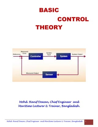
  • 7. Mohd. Hanif Dewan, Chief Engineer and Maritime Lecturer & Trainer, Bangladesh 7 Fig. 1.3 Simple manual temperature control Assessing safety, stability and accuracy Whilst manual operation could probably control the water level in Example 1.1, the manual control of temperature is inherently more difficult in Example 1.3 for various reasons. If the flow of water varies, conditions will tend to change rapidly due to the large amount of heat held in the steam. The operator's response in changing the position of the steam valve may simply not be quick enough. Even after the valve is closed, the coil will still contain a quantity of residual steam, which will continue to give up its heat by condensing. Anticipating change Experience will help but in general the operator will not be able to anticipate change. He must observe change before making a decision and performing an action. This and other factors, such as the inconvenience and cost of a human operator permanently on duty, potential operator error, variations in process needs, accuracy, rapid changes in conditions and the involvement of several processes, all lead to the need for automatic controls. With regards to safety, an audible alarm has been introduced in Example 1.3 to warn of over temperature - another reason for automatic controls. Automatic control A controlled condition might be temperature, pressure, humidity, level, or flow. This means that the measuring element could be a temperature sensor, a pressure transducer or transmitter, a level detector, a humidity sensor or a flow sensor. The manipulated variable could be steam, water, air, electricity, oil or gas, whilst the controlled device could be a valve, damper, pump or fan. For the purposes of demonstrating the basic principles, this Tutorial will concentrate on valves as the controlled device and temperature as the controlled condition, with temperature sensors as the measuring element. Components of an automatic control Figure 1.4 illustrates the component parts of a basic control system. The sensor signals to the controller. The controller, which may take signals from more than one sensor, determines whether a change is required in the manipulated variable, based on these signal(s). It then commands the actuator to move the valve to a different position; more open or more closed depending on the requirement.
  • 8. Mohd. Hanif Dewan, Chief Engineer and Maritime Lecturer & Trainer, Bangladesh 8 Fig. 1.4 Components of an automatic control Controllers are generally classified by the sources of energy that power them, electrical, pneumatic, hydraulic or mechanical. An actuator can be thought of as a motor. Actuators are also classified by the sources of energy that power them, in the same way as controllers. Valves are classified by the action they use to effect an opening or closing of the flow orifice, and by their body configurations, for example whether they consist of a sliding spindle or have a rotary movement. If the system elements are combined with the system parts (or devices) the relationship between 'What needs to be done?' with 'How does it do it?', can be seen. Some of the terms used may not yet be familiar. However, in the following parts of Block 5, all the individual components and items shown on the previous drawing will be addressed. Fig. 1.5 Typical mix of process control devices with system elements
  • 9. Mohd. Hanif Dewan, Chief Engineer and Maritime Lecturer & Trainer, Bangladesh 9 Basic Control Theory Modes of control An automatic temperature control might consist of a valve, actuator, controller and sensor detecting the space temperature in a room. The control system is said to be 'in balance' when the space temperature sensor does not register more or less temperature than that required by the control system. What happens to the control valve when the space sensor registers a change in temperature (a temperature deviation) depends on the type of control system used. The relationship between the movement of the valve and the change of temperature in the controlled medium is known as the mode of control or control action. There are two basic modes of control: 1. On/Off - The valve is either fully open or fully closed, with no intermediate state. 2. Continuous - The valve can move between fully open or fully closed, or be held at any intermediate position. Variations of both these modes exist, which will now be examined in greater detail. 1. On/off control Occasionally known as two-step or two-position control, this is the most basic control mode. Considering the tank of water shown in Figure 2.1, the objective is to heat the water in the tank using the energy given off a simple steam coil. In the flow pipe to the coil, a two port valve and actuator is fitted, complete with a thermostat, placed in the water in the tank. Fig. 2.1 On/off temperature control of water in a tank The thermostat is set to 60°C, which is the required temperature of the water in the tank. Logic dictates that if the switching point were actually at 60°C the system would never operate properly,
  • 10. Mohd. Hanif Dewan, Chief Engineer and Maritime Lecturer & Trainer, Bangladesh 10 because the valve would not know whether to be open or closed at 60°C. From then on it could open and shut rapidly, causing wear. For this reason, the thermostat would have an upper and lower switching point. This is essential to prevent over-rapid cycling. In this case the upper switching point might be 61°C (the point at which the thermostat tells the valve to shut) and the lower switching point might be 59°C (the point when the valve is told to open). Thus there is an in-built switching difference in the thermostat of ±1°C about the 60°C set point. This 2°C (±1°C) is known as the switching differential. (This will vary between thermostats). A diagram of the switching action of the thermostat would look like the graph shown in Figure 2.2. The temperature of the tank contents will fall to 59°C before the valve is asked to open and will rise to 61°C before the valve is instructed to close. Fig. 2.2 On/off switching action of the thermostat Figure 2.2 shows straight switching lines but the effect on heat transfer from coil to water will not be immediate. It will take time for the steam in the coil to affect the temperature of the water in the tank. Not only that, but the water in the tank will rise above the 61°C upper limit and fall below the 59°C lower limit. This can be explained by cross referencing Figures 2.2 and 2.3. First however it is necessary to describe what is happening. At point A (59°C, Figure 2.3) the thermostat switches on, directing the valve wide open. It takes time for the transfer of heat from the coil to affect the water temperature, as shown by the graph of the water temperature in Figure 2.3. At point B (61°C) the thermostat switches off and allows the valve to shut. However the coil is still full of steam, which continues to condense and give up its heat. Hence the water temperature continues to rise above the upper switching temperature, and 'overshoots' at C, before eventually falling.
  • 11. Mohd. Hanif Dewan, Chief Engineer and Maritime Lecturer & Trainer, Bangladesh 11 Fig. 2.3 Tank temperature versus time From this point onwards, the water temperature in the tank continues to fall until, at point D (59°C), the thermostat tells the valve to open. Steam is admitted through the coil but again, it takes time to have an effect and the water temperature continues to fall for a while, reaching its trough of undershoot at point E. The difference between the peak and the trough is known as the operating differential. The switching differential of the thermostat depends on the type of thermostat used. The operating differential depends on the characteristics of the application such as the tank, its contents, the heat transfer characteristics of the coil, the rate at which heat is transferred to the thermostat, and so on. Essentially, with on/off control, there are upper and lower switching limits, and the valve is either fully open or fully closed - there is no intermediate state. However, controllers are available that provide a proportioning time control, in which it is possible to alter the ratio of the 'on' time to the 'off' time to control the controlled condition. This proportioning action occurs within a selected bandwidth around the set point; the set point being the bandwidth mid point. If the controlled condition is outside the bandwidth, the output signal from the controller is either fully on or fully off, acting as an on/off device. If the controlled condition is within the bandwidth, the controller output is turned on and off relative to the deviation between the value of the controlled condition and the set point. With the controlled condition being at set point, the ratio of 'on' time to 'off' time is 1:1, that is, the 'on' time equals the 'off' time. If the controlled condition is below the set point, the 'on' time will be longer than the 'off' time, whilst if above the set point, the 'off' time will be longer, relative to the deviation within the bandwidth. The main advantages of on/off control are that it is simple and very low cost. This is why it is frequently found on domestic type applications such as central heating boilers and heater fans. Its major disadvantage is that the operating differential might fall outside the control tolerance required by the process. For example, on a food production line, where the taste and repeatability of taste is determined by precise temperature control, on/off control could well be unsuitable. By contrast, in the case of space heating there are often large storage capacities (a large area to heat or cool that will respond to temperature change slowly) and slight variation in the desired value is acceptable. In many cases on/off control is quite appropriate for this type of application. If on/off control is unsuitable because more accurate temperature control is required, the next option is continuous control. 2. Continuous control Continuous control is often called modulating control. It means that the valve is capable of moving continually to change the degree of valve opening or closing. It does not just move to either fully open or fully closed, as with on-off control.
  • 12. Mohd. Hanif Dewan, Chief Engineer and Maritime Lecturer & Trainer, Bangladesh 12 There are three basic control actions that are often applied to continuous control: 1. Proportional (P) 2. Integral (I) 3. Derivative (D) It is also necessary to consider these in combination such as P + I, P + D, P + I + D. Although it is possible to combine the different actions, and all help to produce the required response, it is important to remember that both the integral and derivative actions are usually corrective functions of a basic proportional control action. The three control actions are considered below. 1. Proportional control This is the most basic of the continuous control modes and is usually referred to by use of the letter 'P'. The principle aim of proportional control is to control the process as the conditions change. This section shows that:  The larger the proportional band, the more stable the control, but the greater the offset.  The narrower the proportional band, the less stable the process, but the smaller the offset. The aim, therefore, should be to introduce the smallest acceptable proportional band that will always keep the process stable with the minimum offset. In explaining proportional control, several new terms must be introduced. To define these, a simple analogy can be considered - a cold water tank is supplied with water via a float operated control valve and with a globe valve on the outlet pipe valve 'V', as shown in Fig. 2.4. Both valves are the same size and have the same flow capacity and flow characteristic. The desired water level in the tank is at point B (equivalent to the set point of a level controller). It can be assumed that, with valve 'V' half open, (50% load) there is just the right flowrate of water entering via the float operated valve to provide the desired flow out through the discharge pipe, and to maintain the water level in the tank at point at B. The questions these people ask about steam are markedly different.
  • 13. Mohd. Hanif Dewan, Chief Engineer and Maritime Lecturer & Trainer, Bangladesh 13 Fig. 2.4 Valve 50% open The system can be said to be in balance (the flowrate of water entering and leaving the tank is the same); under control, in a stable condition (the level is not varying) and at precisely the desired water level (B ); giving the required outflow. With the valve 'V' closed, the level of water in the tank rises to point A and the float operated valve cuts off the water supply (see Fig. 2.5 below). The system is still under control and stable but control is above level B. The difference between level B and the actual controlled level, A, is related to the proportional band of the control system. Once again, if valve 'V' is half opened to give 50% load, the water level in the tank will return to the Desired level, point B. Fig. 2.5 Valve closed This means the system is simpler and less expensive than, for example, a high temperature hot water system. The high efficiency of steam plant means it is compact and makes maximum use of space, something which is often at a premium within plant. Furthermore, upgrading an existing steam system with the latest boilers and controls typically represents 50% of the cost of removing it and replacing it with a decentralised gas fired system. Fig. 2.6 Valve open The system is under control and stable, but there is an offset; the deviation in level between points B and C. Figure 2.7 combines the three conditions used in this example.
  • 14. Mohd. Hanif Dewan, Chief Engineer and Maritime Lecturer & Trainer, Bangladesh 14 The difference in levels between points A and C is known as the Proportional Band or P-band, since this is the change in level (or temperature in the case of a temperature control) for the control valve to move from fully open to fully closed. One recognised symbol for Proportional Band is Xp. The analogy illustrates several basic and important points relating to proportional control:  The control valve is moved in proportion to the error in the water level (or the temperature deviation, in the case of a temperature control) from the set point.  The set point can only be maintained for one specific load condition.  Whilst stable control will be achieved between points A and C, any load causing a difference in level to that of B will always provide an offset. Fig. 2.7 Proportional band Note: By altering the fulcrum position, the system Proportional Band changes. Nearer the float gives a narrower P-band, whilst nearer the valve gives a wider P-band. Fig. 2.8 illustrates why this is so. Different fulcrum positions require different changes in water level to move the valve from fully open to fully closed. In both cases, It can be seen that level B represents the 50% load level, A represents the 0% load level, and C represents the 100% load level. It can also be seen how the offset is greater at any same load with the wider proportional band. Fig. 2.8 Demonstrating the relationship between P-band and offset
  • 15. Mohd. Hanif Dewan, Chief Engineer and Maritime Lecturer & Trainer, Bangladesh 15 The examples depicted in Fig. 2.4 through to 2.8 describe proportional band as the level (or perhaps temperature or pressure etc.) change required to move the valve from fully open to fully closed. This is convenient for mechanical systems, but a more general (and more correct) definition of proportional band is the percentage change in measured value required to give a 100% change in output. It is therefore usually expressed in percentage terms rather than in engineering units such as degrees centigrade. For electrical and pneumatic controllers, the set value is at the middle of the proportional band. The effect of changing the P-band for an electrical or pneumatic system can be described with a slightly different example, by using a temperature control. The space temperature of a building is controlled by a water (radiator type) heating system using a proportional action control by a valve driven with an electrical actuator, and an electronic controller and room temperature sensor. The control selected has a proportional band (P-band or Xp) of 6% of the controller input span of 0° - 100°C, and the desired internal space temperature is 18°C. Under certain load conditions, the valve is 50% open and the required internal temperature is correct at 18°C. A fall in outside temperature occurs, resulting in an increase in the rate of heat loss from the building. Consequently, the internal temperature will decrease. This will be detected by the room temperature sensor, which will signal the valve to move to a more open position allowing hotter water to pass through the room radiators. The valve is instructed to open by an amount proportional to the drop in room temperature. In simplistic terms, if the room temperature falls by 1°C, the valve may open by 10%; if the room temperature falls by 2°C, the valve will open by 20%. In due course, the outside temperature stabilises and the inside temperature stops falling. In order to provide the additional heat required for the lower outside temperature, the valve will stabilise in a more open position; but the actual inside temperature will be slightly lower than 18°C. Example 2.1 and Fig. 2.9 explain this further, using a P-band of 6°C. Example 2.1 Consider a space heating application with the following characteristics: 1. The required temperature in the building is 18°C. 2. The room temperature is currently 18°C, and the valve is 50% open. 3. The proportional band is set at 6% of 100°C = 6°C, which gives 3°C either side of the 18°C set point.
  • 16. Mohd. Hanif Dewan, Chief Engineer and Maritime Lecturer & Trainer, Bangladesh 16 Figure 2.9 shows the room temperature and valve relationship: Fig. 2.9 Room temperature and valve relationship - 6°C proportional band As an example, consider the room temperature falling to 16°C. From the chart it can be seen that the new valve opening will be approximately 83%. With proportional control, if the load changes, so too will the offset:  A load of less than 50% will cause the room temperature to be above the set value.  A load of more than 50% will cause the room temperature to be below the set value. The deviation between the set temperature on the controller (the set point) and the actual room temperature is called the 'proportional offset'. In Example 2.1, as long as the load conditions remain the same, the control will remain steady at a valve opening of 83.3%; this is called 'sustained offset'. The effect of adjusting the P-band In electronic and pneumatic controllers, the P-band is adjustable. This enables the user to find a setting suitable for the individual application. Increasing the P-band - For example, if the previous application had been programmed with a 12% proportional band equivalent to 12°C, the results can be seen in Fig. 2.10. Note that the wider P-band results in a less steep 'gain' line. For the same change in room temperature the valve movement will be smaller. The term 'gain' is discussed in a following section. In this instance, the 2°C fall in room temperature would give a valve opening of about 68% from the chart in Fig. 2.10.
  • 17. Mohd. Hanif Dewan, Chief Engineer and Maritime Lecturer & Trainer, Bangladesh 17 Fig. 2.10 Room temperature and valve relationship - 12°C Proportional band Reducing the P-band - Conversely, if the P-band is reduced, the valve movement per temperature increment is increased. However, reducing the P-band to zero gives an on/off control. The ideal P- band is as narrow as possible without producing a noticeable oscillation in the actual room temperature. Example 2.2 Let the input span of a controller be 100°C. If the controller is set so that full change in output occurs over a proportional band of 20% the controller gain is: Gain The term 'gain' is often used with controllers and is simply the reciprocal of proportional band. The larger the controller gain, the more the controller output will change for a given error. For instance for a gain of 1, an error of 10% of scale will change the controller output by 10% of scale, for a gain of 5, an error of 10% will change the controller output by 50% of scale, whilst for a gain of 10, an error of 10% will change the output by 100% of scale. The proportional band in 'degree terms' will depend on the controller input scale. For instance, for a controller with a 200°C input scale: An Xp of 20% = 20% of 200°C = 40°C An Xp of 10% = 10% of 200°C = 20°C
  • 18. Mohd. Hanif Dewan, Chief Engineer and Maritime Lecturer & Trainer, Bangladesh 18 Example 2.2 Let the input span of a controller be 100°C. If the controller is set so that full change in output occurs over a proportional band of 20% the controller gain is: Equally it could be said that the proportional band is 20% of 100°C = 20°C and the gain is: Therefore the relationship between P-band and Gain is: As a reminder:  A wide proportional band (small gain) will provide a less sensitive response, but a greater stability.  A narrow proportional band (large gain) will provide a more sensitive response, but there is a practical limit to how narrow the Xp can be set.  Too narrow a proportional band (too much gain) will result in oscillation and unstable control. For any controller for various P-bands, gain lines can be determined as shown in Fig. 2.11, where the controller input span is 100°C.
  • 19. Mohd. Hanif Dewan, Chief Engineer and Maritime Lecturer & Trainer, Bangladesh 19 Fig. 2.11 Proportional band and gain Reverse or direct acting control signal A closer look at the figures used so far to describe the effect of proportional control shows that the output is assumed to be reverse acting. In other words, a rise in process temperature causes the control signal to fall and the valve to close. This is usually the situation on heating controls. This configuration would not work on a cooling control; here the valve must open with a rise in temperature. This is termed a direct acting control signal. Fig. 2.12 and 2.13 depict the difference between reverse and direct acting control signals for the same valve action. Fig. 2.12 Reverse acting signal
  • 20. Mohd. Hanif Dewan, Chief Engineer and Maritime Lecturer & Trainer, Bangladesh 20 Fig. 2.13 Direct acting signal On mechanical controllers (such as a pneumatic controller) it is usual to be able to invert the output signal of the controller by rotating the proportional control dial. Thus, the magnitude of the proportional band and the direction of the control action can be determined from the same dial. On electronic controllers, reverse acting (RA) or direct acting (DA) is selected through the keypad. Gain line offset or proportional effect From the explanation of proportional control, it should be clear that there is a control offset or a deviation of the actual value from the set value whenever the load varies from 50%. To further illustrate this, consider Example 2.1 with a 12°C P-band, where an offset of 2°C was expected. If the offset cannot be tolerated by the application, then it must be eliminated. This could be achieved by relocating (or resetting) the set point to a higher value. This provides the same valve opening after manual reset but at a room temperature of 18°C not 16°C.
  • 21. Mohd. Hanif Dewan, Chief Engineer and Maritime Lecturer & Trainer, Bangladesh 21 Fig. 2.14 Gain line offset Manual reset The offset can be removed either manually or automatically. The effect of manual reset can be seen in Figure 2.14, and the value is adjusted manually by applying an offset to the set point of 2°C. It should be clear from Fig. 2.14 and the above text that the effect is the same as increasing the set value by 2°C. The same valve opening of 66.7% now coincides with the room temperature at 18°C.
  • 22. Mohd. Hanif Dewan, Chief Engineer and Maritime Lecturer & Trainer, Bangladesh 22 The effects of manual reset are demonstrated in Figure 2.15.
  • 23. Mohd. Hanif Dewan, Chief Engineer and Maritime Lecturer & Trainer, Bangladesh 23 Fig. 2.15 Effect of manual reset Integral control - automatic reset action 'Manual reset' is usually unsatisfactory in process plant where each load change will require a reset action. It is also quite common for an operator to be confused by the differences between:  Set value - What is on the dial.  Actual value - What the process value is.  Required value - The perfect process condition. Such problems are overcome by the reset action being contained within the mechanism of an automatic controller. Such a controller is primarily a proportional controller. It then has a reset function added, which is called 'integral action'. Automatic reset uses an electronic or pneumatic integration routine to perform the reset function. The most commonly used term for automatic reset is integral action, which is given the letter I. The function of integral action is to eliminate offset by continuously and automatically modifying the controller output in accordance with the control deviation integrated over time. The Integral Action Time (IAT) is defined as the time taken for the controller output to change due to the integral action to equal the output change due to the proportional action. Integral action gives a steadily increasing corrective action as long as an error continues to exist. Such corrective action will increase with time and must therefore, at some time, be sufficient to eliminate the steady state error altogether, providing sufficient time elapses before another change occurs. The controller allows the integral time to be adjusted to suit the plant dynamic behaviour. Proportional plus integral (P + I) becomes the terminology for a controller incorporating these features. The integral action on a controller is often restricted to within the proportional band. A typical P + I response is shown in Fig. 2.16, for a step change in load.
  • 24. Mohd. Hanif Dewan, Chief Engineer and Maritime Lecturer & Trainer, Bangladesh 24 Fig. 2.16 P+I Function after a step change in load The IAT is adjustable within the controller:  If it is too short, over-reaction and instability will result.  If it is too long, reset action will be very slow to take effect. IAT is represented in time units. On some controllers the adjustable parameter for the integral action is termed 'repeats per minute', which is the number of times per minute that the integral action output changes by the proportional output change.  Repeats per minute = 1/(IAT in minutes)  IAT = Infinity - Means no integral action  IAT = 0 - Means infinite integral action It is important to check the controller manual to see how integral action is designated. Overshoot and 'wind up' With P+ I controllers (and with P controllers), overshoot is likely to occur when there are time lags on the system. A typical example of this is after a sudden change in load. Consider a process application where a process heat exchanger is designed to maintain water at a fixed temperature. The set point is 80°C, the P-band is set at 5°C (±2.5°C), and the load suddenly changes such that the returning water temperature falls almost instantaneously to 60°C. Figure 2.16 shows the effect of this sudden (step change) in load on the actual water temperature. The measured value changes almost instantaneously from a steady 80°C to a value of 60°C. By the nature of the integration process, the generation of integral control action must lag behind the proportional control action, introducing a delay and more dead time to the response. This could have
  • 25. Mohd. Hanif Dewan, Chief Engineer and Maritime Lecturer & Trainer, Bangladesh 25 serious consequences in practice, because it means that the initial control response, which in a proportional system would be instantaneous and fast acting, is now subjected to a delay and responds slowly. This may cause the actual value to run out of control and the system to oscillate. These oscillations may increase or decrease depending on the relative values of the controller gain and the integral action. If applying integral action it is important to make sure, that it is necessary and if so, that the correct amount of integral action is applied. Integral control can also aggravate other situations. If the error is large for a long period, for example after a large step change or the system being shut down, the value of the integral can become excessively large and cause overshoot or undershoot that takes a long time to recover. To avoid this problem, which is often called 'integral wind-up', sophisticated controllers will inhibit integral action until the system gets fairly close to equilibrium. To remedy these situations it is useful to measure the rate at which the actual temperature is changing; in other words, to measure the rate of change of the signal. Another type of control mode is used to measure how fast the measured value changes, and this is termed Rate Action or Derivative Action. Derivative control - rate action A Derivative action (referred to by the letter D) measures and responds to the rate of change of process signal, and adjusts the output of the controller to minimise overshoot. If applied properly on systems with time lags, derivative action will minimise the deviation from the set point when there is a change in the process condition. It is interesting to note that derivative action will only apply itself when there is a change in process signal. If the value is steady, whatever the offset, then derivative action does not occur. One useful function of the derivative function is that overshoot can be minimised especially on fast changes in load. However, derivative action is not easy to apply properly; if not enough is used, little benefit is achieved, and applying too much can cause more problems than it solves. D action is again adjustable within the controller, and referred to as TD in time units: T D = 0 - Means no D action. T D = Infinity - Means infinite D action. P + D controllers can be obtained, but proportional offset will probably be experienced. It is worth remembering that the main disadvantage with a P control is the presence of offset. To overcome and remove offset, 'I' action is introduced. The frequent existence of time lags in the control loop explains the need for the third action D. The result is a P + I + D controller which, if properly tuned, can in most processes give a rapid and stable response, with no offset and without overshoot.
  • 26. Mohd. Hanif Dewan, Chief Engineer and Maritime Lecturer & Trainer, Bangladesh 26 PID controllers P and I and D are referred to as 'terms' and thus a P + I + D controller is often referred to as a three term controller. Summary of modes of control A three-term controller contains three modes of control:  Proportional (P) action with adjustable gain to obtain stability.  Reset (Integral) (I) action to compensate for offset due to load changes.  Rate (Derivative) (D) action to speed up valve movement when rapid load changes take place. The various characteristics can be summarised, as shown in Fig. 2.17. Fig. 2.17 Summary of control modes and responses
  • 27. Mohd. Hanif Dewan, Chief Engineer and Maritime Lecturer & Trainer, Bangladesh 27 Finally, the controls engineer must try to avoid the danger of using unnecessarily complicated controls for a specific application. The least complicated control action, which will provide the degree of control required, should always be selected. Further terminology Time constant This is defined as: 'The time taken for a controller output to change by 63.2% of its total due to a step (or sudden) change in process load'. In reality, the explanation is more involved because the time constant is really the time taken for a signal or output to achieve its final value from its initial value, had the original rate of increase been maintained. This concept is depicted in Fig. 12.18. Fig. 2.18 Time constant Example 2.2 A practical appreciation of the time constant Consider two tanks of water, tank A at a temperature of 25°C, and tank B at 75°C. A sensor is placed in tank A and allowed to reach equilibrium temperature. It is then quickly transferred to tank B. The temperature difference between the two tanks is 50°C, and 63.2% of this temperature span can be calculated as shown below: 63.2% of 50°C = 31.6°C The initial datum temperature was 25°C, consequently the time constant for this simple example is the time required for the sensor to reach 56.6°C, as shown below:
  • 28. Mohd. Hanif Dewan, Chief Engineer and Maritime Lecturer & Trainer, Bangladesh 28 25°C + 31.6°C = 56.6°C Hunting Often referred to as instability, cycling or oscillation. Hunting produces a continuously changing deviation from the normal operating point. This can be caused by: Hunting  The proportional band being too narrow.  The integral time being too short.  The derivative time being too long.  A combination of these.  Long time constants or dead times in the control system or the process itself. In Fig. 2.19 the heat exchanger is oversized for the application. Accurate temperature control will be difficult to achieve and may result in a large proportional band in an attempt to achieve stability. If the system load suddenly increases, the two port valve will open wider, filling the heat exchanger with high temperature steam. The heat transfer rate increases extremely quickly causing the water system temperature to overshoot. The rapid increase in water temperature is picked up by the sensor and directs the two port valve to close quickly. This causes the water temperature to fall, and the two port valve to open again. This cycle is repeated, the cycling only ceasing when the PID terms are adjusted. The following example (Example 2.3) gives an idea of the effects of a hunting steam system.
  • 29. Mohd. Hanif Dewan, Chief Engineer and Maritime Lecturer & Trainer, Bangladesh 29 Fig. 2.19 Hunting Example 2.3 The effect of hunting on the system in Fig. 2.19 Consider the steam to water heat exchanger system in Fig. 2.19. Under minimum load conditions, the size of the heat exchanger is such that it heats the constant flowrate secondary water from 60°C to 65°C with a steam temperature of 70°C. The controller has a set point of 65°C and a P-band of 10°C. Consider a sudden increase in the secondary load, such that the returning water temperature almost immediately drops by 40°C. The temperature of the water flowing out of the heat exchanger will also drop by 40°C to 25°C. The sensor detects this and, as this temperature is below the P-band, it directs the pneumatically actuated steam valve to open fully. The steam temperature is observed to increase from 70°C to 140°C almost instantaneously. What is the effect on the secondary water temperature and the stability of the control system? the heat exchanger temperature design constant, TDC, can be calculated from the observed operating conditions and Equation 2.2 Equation 2.2 Where: TDC = Temperature Design Constant T s = Steam temperature T 1 = Secondary fluid inlet temperature T 2 = Secondary fluid outlet temperature In this example, the observed conditions (at minimum load) are as follows:
  • 30. Mohd. Hanif Dewan, Chief Engineer and Maritime Lecturer & Trainer, Bangladesh 30 When the steam temperature rises to 140°C, it is possible to predict the outlet temperature from Equation 2.3: Equation 2.3 Where: T s = 140°C T 1 = 60°C - 40°C = 20°C temperature TDC = 2 The heat exchanger outlet temperature is 80°C, which is now above the P-band, and the sensor now signals the controller to shut down the steam valve. The steam temperature falls rapidly, causing the outlet water temperature to fall; and the steam valve opens yet again. The system cycles around these temperatures until the control parameters are changed. These symptoms are referred to as 'hunting'. The control valve and its controller are hunting to find a stable condition. In practice, other factors will add to the uncertainty of the situation, such as the system size and reaction to temperature change and the position of the sensor. Hunting of this type can cause premature wear of system components, in particular valves and actuators, and gives poor control. Example 2.3 is not typical of a practical application. In reality, correct design and sizing of the control system and steam heated heat exchanger would not be a problem. Lag Lag is a delay in response and will exist in both the control system and in the process or system under control. Consider a small room warmed by a heater, which is controlled by a room space thermostat. A large window is opened admitting large amounts of cold air. The room temperature will fall but there will be a delay while the mass of the sensor cools down to the new temperature - this is known as control lag. The delay time is also referred to as dead time. Having then asked for more heat from the room heater, it will be some time before this takes effect
  • 31. Mohd. Hanif Dewan, Chief Engineer and Maritime Lecturer & Trainer, Bangladesh 31 and warms up the room to the point where the thermostat is satisfied. This is known as system lag or thermal lag. Rangeability This relates to the control valve and is the ratio between the maximum controllable flow and the minimum controllable flow, between which the characteristics of the valve (linear, equal percentage, quick opening) will be maintained. With most control valves, at some point before the fully closed position is reached, there is no longer a defined control over flow in accordance with the valve characteristics. Reputable manufacturers will provide rangeability figures for their valves. Turndown ratio Turndown ratio is the ratio between the maximum flow and the minimum controllable flow. It will be substantially less than the valve's rangeability if the valve is oversized. Although the definition relates only to the valve, it is a function of the complete control system. Control Loops and Dynamics Control loops An open loop control system Open loop control simply means there is no direct feedback from the controlled condition; in other words, no information is sent back from the process or system under control to advise the controller that corrective action is required. The heating system shown in Figure 5.3.1 demonstrates this by using a sensor outside of the room being heated. The system shown in Figure 5.3.1 is not an example of a practical heating control system; it is simply being used to depict the principle of open loop control. Fig. 3.1 Open loop control The system consists of a proportional controller with an outside sensor sensing ambient air temperature. The controller might be set with a fairly large proportional band, such that at an ambient
  • 32. Mohd. Hanif Dewan, Chief Engineer and Maritime Lecturer & Trainer, Bangladesh 32 temperature of -1°C the valve is full open, and at an ambient of 19°C the valve is fully closed. As the ambient temperature will have an effect on the heat loss from the building, it is hoped that the room temperature will be controlled. However, there is no feedback regarding the room temperature and heating due to other factors. In mild weather, although the flow of water is being controlled, other factors, such as high solar gain, might cause the room to overheat. In other words, open control tends only to provide a coarse control of the application. Fig. 3.2 depicts a slightly more sophisticated control system with two sensors. Fig. 3.2 Open loop control system with outside temperature sensor and water temperature sensor The system uses a three port mixing valve with an actuator, controller and outside air sensor, plus a temperature sensor in the water line. The outside temperature sensor provides a remote set point input to the controller, which is used to offset the water temperature set point. In this way, closed loop control applies to the water temperature flowing through the radiators. When it is cold outside, water flows through the radiator at its maximum temperature. As the outside temperature rises, the controller automatically reduces the temperature of the water flowing through the radiators. However, this is still open loop control as far as the room temperature is concerned, as there is no feedback from the building or space being heated. If radiators are oversized or design errors have occurred, overheating will still occur. Closed loop control Quite simply, a closed loop control requires feedback; information sent back direct from the process or system. Using the simple heating system shown in Figure 5.3.3, the addition of an internal space temperature sensor will detect the room temperature and provide closed loop control with respect to the room.
  • 33. Mohd. Hanif Dewan, Chief Engineer and Maritime Lecturer & Trainer, Bangladesh 33 In Fig. 3.3, the valve and actuator are controlled via a space temperature sensor in the room, providing feedback from the actual room temperature. Fig.3.3 Closed loop control system with sensor for internal space temperature Disturbances Disturbances are factors, which enter the process or system to upset the value of the controlled medium. These disturbances can be caused by changes in load or by outside influences. For example; if in a simple heating system, a room was suddenly filled with people, this would constitute a disturbance, since it would affect the temperature of the room and the amount of heat required to maintain the desired space temperature. Feedback control This is another type of closed loop control. Feedback control takes account of disturbances and feeds this information back to the controller, to allow corrective action to be taken. For example, if a large number of people enter a room, the space temperature will increase, which will then cause the control system to reduce the heat input to the room. Feed-forward control With feed-forward control, the effects of any disturbances are anticipated and allowed for before the event actually takes place. An example of this is bringing the boiler up to high fire before bringing a large steam-using process plant on line. The sequence of events might be that the process plant is switched on. This action, rather than opening the steam valve to the process, instructs the boiler burner to high fire. Only when
  • 34. Mohd. Hanif Dewan, Chief Engineer and Maritime Lecturer & Trainer, Bangladesh 34 the high fire position is reached is the process steam valve allowed to open, and then in a slow, controlled way. Single loop control This is the simplest control loop involving just one controlled variable, for instance, temperature. To explain this, a steam-to-water heat exchanger is considered as shown in Fig. 3.4. Fig. 3.4 Single loop control on a heating calorifier The only one variable controlled in Figure 3.4 is the temperature of the water leaving the heat exchanger. This is achieved by controlling the 2-port steam valve supplying steam to the heat exchanger. The primary sensor may be a thermocouple or PT100 platinum resistance thermometer sensing the water temperature. The controller compares the signal from the sensor to the set point on the controller. If there is a difference, the controller sends a signal to the actuator of the valve, which in turn moves the valve to a new position. The controller may also include an output indicator, which shows the percentage of valve opening. Single control loops provide the vast majority of control for heating systems and industrial processes. Other terms used for single control loops include:  Set value control.  Single closed loop control.
  • 35. Mohd. Hanif Dewan, Chief Engineer and Maritime Lecturer & Trainer, Bangladesh 35  Feedback control. Multi-loop control The following example considers an application for a slow moving timber-based product, which must be controlled to a specific humidity level (see Fig. 3.5 and 3.6). Fig. 3.5 Single humidity sensor In Fig. 3.5, the single humidity sensor at the end of the conveyor controls the amount of heat added by the furnace. But if the water spray rate changes due, for instance, to fluctuations in the water supply pressure, it may take perhaps 10 minutes before the product reaches the far end of the conveyor and the humidity sensor reacts. This will cause variations in product quality. To improve the control, a second humidity sensor on another control loop can be installed immediately after the water spray, as shown in Fig. 3.6. This humidity sensor provides a remote set point input to the controller which is used to offset the local set point. The local set point is set at the required humidity after the furnace. This, in a simple form, illustrates multi-loop control. This humidity control system consists of two control loops:  Loop 1 controls the addition of water.  Loop 2 controls the removal of water. Within this process, factors will influence both loops. Some factors such as water pressure will affect both loops. Loop 1 will try to correct for this, but any resulting error will have an impact on Loop 2.
  • 36. Mohd. Hanif Dewan, Chief Engineer and Maritime Lecturer & Trainer, Bangladesh 36 Fig. 3.6 Dual humidity sensors Cascade control Where two independent variables need to be controlled with one valve, a cascade control system may be used. Figure 3.7 shows a steam jacketed vessel full of liquid product. The essential aspects of the process are quite rigorous:  The product in the vessel must be heated to a certain temperature.  The steam must not exceed a certain temperature or the product may be spoiled.  The product temperature must not increase faster than a certain rate or the product may be spoiled. If a normal, single loop control was used with the sensor in the liquid, at the start of the process the sensor would detect a low temperature, and the controller would signal the valve to move to the fully open position. This would result in a problem caused by an excessive steam temperature in the jacket.
  • 37. Mohd. Hanif Dewan, Chief Engineer and Maritime Lecturer & Trainer, Bangladesh 37 Fig. 3.7 Jacketed vessel The solution is to use a cascade control using two controllers and two sensors:  A slave controller (Controller 2) and sensor monitoring the steam temperature in the jacket, and outputting a signal to the control valve.  A master controller (Controller 1) and sensor monitoring the product temperature with the controller output directed to the slave controller.  The output signal from the master controller is used to vary the set point in the slave controller, ensuring that the steam temperature is not exceeded. Example 3.1 An example of cascade control applied to a process vessel The liquid temperature is to be heated from 15°C to 80°C and maintained at 80°C for two hours. The steam temperature cannot exceed 120°C under any circumstances. The product temperature must not increase faster than 1°C/minute. The master controller can be ramped so that the rate of increase in water temperature is not higher than that specified. The master controller is set in reverse acting mode, so that its output signal to the slave controller is 20 mA at low temperature and 4 mA at high temperature. The remote set point on the slave controller is set so that its output signal to the valve is 4 mA when the steam temperature is 80°C, and 20 mA when the steam temperature is 120°C. In this way, the temperature of the steam cannot be higher than that tolerated by the system, and the steam pressure in the jacket cannot be higher than the, 1 bar g, saturation pressure at 120°C. Dynamics of the process This is a very complex subject but this part of the text will cover the most basic considerations. It is the time taken for a control system to reach approximately two-thirds of its total movement as a result of a given step change in temperature, or other variable. Other parts of the control system will have similar time based responses - the controller and its components and the sensor itself. All instruments have a time lag between the input to the instrument and its subsequent output. Even the transmission system will have a time lag - not a problem with electric/electronic systems but a factor that may need to be taken into account with pneumatic transmission systems. Fig. 3.8 and 3.9 show some typical response lags for a thermocouple that has been installed into a pocket for sensing water temperature.
  • 38. Mohd. Hanif Dewan, Chief Engineer and Maritime Lecturer & Trainer, Bangladesh 38 Fig. 3.8 Step change 5°C Fig. 3.9 Ramp change 5°C Apart from the delays in sensor response, other parts of the control system also affect the response time. With pneumatic and self-acting systems, the valve/actuator movement tends to be smooth and, in a proportional controller, directly proportional to the temperature deviation at the sensor. With an electric actuator there is a delay due to the time it takes for the motor to move the control linkage. Because the control signal is a series of pulses, the motor provides bursts of movement followed by periods where the actuator is stationary. The response diagram (Fig. 3.10) depicts this. However, because of delays in the process response, the final controlled temperature can still be smooth. Fig. 3.10 Comparison of response by different actuators
  • 39. Mohd. Hanif Dewan, Chief Engineer and Maritime Lecturer & Trainer, Bangladesh 39 The control systems covered in this Tutorial have only considered steady state conditions. However the process or plant under control may be subject to variations following a certain behaviour pattern. The control system is required to make the process behave in a predictable manner. If the process is one which changes rapidly, then the control system must be able to react quickly. If the process undergoes slow change, the demands on the operating speed of the control system are not so stringent. Much is documented about the static and dynamic behaviour of controllers and control systems - sensitivity, response time and so on. Possibly the most important factor of consideration is the time lag of the complete control loop. The dynamics of the process need consideration to select the right type of controller, sensor and actuator. Process reactions These dynamic characteristics are defined by the reaction of the process to a sudden change in the control settings, known as a step input. This might include an immediate change in set temperature, as shown in Figure 3.11. The response of the system is depicted in Figure 3.12, which shows a certain amount of dead time before the process temperature starts to increase. This dead time is due to the control lag caused by such things as an electrical actuator moving to its new position. The time constant will differ according to the dynamic response of the system, affected by such things as whether or not the sensor is housed in a pocket. Fig. 3.11 Step input
  • 40. Mohd. Hanif Dewan, Chief Engineer and Maritime Lecturer & Trainer, Bangladesh 40 Fig. 3.12 Components of process response to step changes The response of any two processes can have different characteristics because of the system. The effects of dead time and the time constant on the system response to a sudden input change are shown graphically in Fig. 3.12. Systems that have a quick initial rate of response to input changes are generally referred to as possessing a first order response. Systems that have a slow initial rate of response to input changes are generally referred to as possessing a second order response. An overview of the basic types of process response (effects of dead time, first order response, and second order response) is shown in Fig. 3.13. Fig. 3.13 Response curves (Reference: spirax sarco)