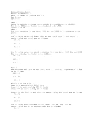
1. Command Window Output
Michael Mastromichalis
Aero 2200 DA-40 Performance Analysis
Dr. Gregory
11/16/2013
Task 1.
Using the methods in class, the parasitic drag coefficient is .0.0398.
The Oswald Efficiency Factor was calculated to be .763.
L/Dmax is 14.38.
Task 2
The power required for sea level, 5000 ft, and 10000 ft is indicated on the
graph.
The following values for stall speed at sea level, 5000 ft, and 10000 ft,
respectively, (in knots) are as follows:
53.1252
57.2295
61.8149
The following values for speed at minimum PR at sea level, 5000 ft, and 10000
ft, respectively, (in knots) are as follows:
101.1038
108.9147
117.6413
Task 3
Maximum power available at sea level, 5000 ft, 10000 ft, respectively,(in hp)
is as follows:
132.7560
110.6300
88.5040
According to the graph...
Vmax_SL is approximately 137.7 knots
Vmax_5000 is apporximately 133.825 knots
Vmax_10000 is approximately 126.32 knots
VTRmin for SL, 5000 ft, and 10000 ft, respectively, (in knots) are as follows
75.8672
81.7284
88.2768
The following Power Required for sea level, 5000 ft, and 10000 ft,
respectively, (in hp) at minimum speed are as follows:
31.3137

2. 33.7329
36.4357
The following Power Available for sea level, 5000 ft, and 10000 ft,
respectively, (in hp) at minimum speed are as follows:
123.5745
104.9177
85.3150
The following Power Required for sea level, 5000 ft, and 10000 ft,
respectively, (in hp) at L/Dmax are as follows:
58.8536
63.4004
68.4803
The following Power Available for sea level, 5000 ft, and 10000 ft,
respectively, (in hp) at L/Dmax are as follows:
123.5745
104.9177
85.3150
The following Power Required for sea level, 5000 ft, and 10000 ft,
respectively, (in hp) at Vmmax are as follows:
140.0632
119.4555
99.3369
The following Power Available for sea level, 5000 ft, and 10000 ft,
respectively, (in hp) at Vmax are as follows:
131.3294
108.9971
86.4143
Task 4
The maximum rate of climb values (in knots) for sea level, 5000 ft, and 10000
ft, respectively, are as follows:
8.4267
6.0733

3. 3.5972
From the graph, the absolute ceiling is 17500 ft, and the service ceiling is
15450 ft.
The time to climb (min) is as follows:
17.9224
According to the graph, the Best Climb Angle Condition Rate of Climb is 7.669
knots
The climb angle Best Climb Angle Condition (in degrees is as follows:
6.5298
The velocity for Best Climb Angle Condition (in knots) is as follows:
67.4375
The Rate of Climb (knots fo)r Best Rate of Climb is as follows:
8.4060
According to the graph, the velocity for the Best Rate of Climb Condition is
83.58 knots
The angle for the Best Rate of Climb Condition (in degrees) is as follows:
5.7432
Task 5
The Endurance is 10.25 hours.
The Range is 803.15 nautical miles.
Task 6
The maximum glide distance is 9.47 nauitcal miles.
The indicated airspeed for maximum glide distance is 85.15 knots.
The airspeed for maximum time aloft is 47.92 knots.
The descent time is 0.20 hours.
Task 7
The maneuverability point is located at 103.56 knots.
the minimum turn radius is 0.04 nautical miles.
The maximum turn rate is 23.77 deg/s.
Task 8
The takeoff ground roll distance at maximum takeoff weight at standard sea
level conditions is 1454.51 feet.
The takeoff ground roll distance at maximum takeoff weight at 5000 ft is
1687.93 feet.
The takeoff ground roll distance at 2400 lb at standard sea level conditions
is 1172.26 feet.
The landing ground roll distance at maximum weight at standard sea level
conditions is 1110.43 feet.
>>

4. Graphs

6. Script
clear, clc
disp('Michael Mastromichalis')
disp('Aero 2200 DA-40 Performance Analysis')
disp('Dr. Gregory')
disp('11/16/2013')
disp(' ')
%Determine the power curve for the Diamond DA-40 given takeoff weight, Power
%available, and efficiency.
W = 2645; %lb%
e = .75;
CDo = .0300;
SHP_SL = 180; %hp
SHP_5000 = 150; %hp
SHP_10000 = 120; %hp
S = 145.7; %ft^2
b = 39.17; %ft
AR = (b^2)/S;
CLmax = 1.90;
%Conditions at sea level, 5000 ft, and 10000 ft
rho = 2.3769*(10^-3); %slug/ft^3
rho_5000 = 2.0482 * (10^-3); %slug/ft^3
rho_10000 = 1.7556 * (10^-3); %slug/ft^3

7. disp('Task 1.')
disp('Using the methods in class, the parasitic drag coefficient is
.0.0398.')
disp('The Oswald Efficiency Factor was calculated to be .763.')
%Now find the drag polar
V_stall = sqrt(2*(W/S)/(rho*CLmax));
V_assume = [V_stall : 500]; %ft/s
CL = (2 * W)./(rho .* V_assume.^2 * S);
CD = CDo +((CL.^2)./(pi*e*AR));
figure(1)
C_L_min = min(CL);
plot(C_L_min, CDo, '*')
legend('CDo')
hold on
plot(CL, CD)
title('CD vs. CL')
xlabel('CL')
ylabel('CD')
L_over_D = CL./CD;
figure(2)
plot(CL, L_over_D)
title('L/D vs. CL')
xlabel('CL')
ylabel('L/D')
L_over_D_max = max(L_over_D);
fprintf('L/Dmax is %.2f.' , L_over_D_max)
disp(' ')
disp('Task 2')
disp('The power required for sea level, 5000 ft, and 10000 ft is indicated on
the graph.')
disp(' ')
%To calculate airspeed for PR min
B_SL = W^2/(.5 * rho * S * pi * AR * e);
A_SL = .5 * rho * S * CDo;
B_5000 = W^2/(.5 * rho_5000 * S * pi * AR * e);
A_5000 = .5 * rho_5000 * S * CDo;
B_10000 = W^2/(.5 * rho_10000 * S * pi * AR * e);
A_10000 = .5 * rho_10000 * S * CDo;
%Define a velocity vector and convert it to ft/s for the necessary
%calculations
V = (40:150); %knots
V_calculation = V*6076/3600; %ft/s
%Calculate Power Required
PR_SL = A_SL * V_calculation.^3 + B_SL * V_calculation.^(-1);
PR_5000 = A_5000 * V_calculation.^3 + B_5000 * V_calculation.^(-1);

8. PR_10000 = A_10000 * V_calculation.^3 + B_10000 * V_calculation.^(-1);
%Convert to hp
PR_SL = PR_SL/550; %hp
PR_5000 = PR_5000/550; %hp
PR_10000 = PR_10000/550; %hp
%Calculate Vstall
Vstall_SL = sqrt(2 * W / (rho * S * CLmax));
Vstall_5000 = sqrt(2 * W / (rho_5000 * S * CLmax));
Vstall_10000 = sqrt(2 * W / (rho_10000 * S * CLmax));
%Convert to knots
Vstall_SL = Vstall_SL*3600/6076; %knots
Vstall_5000 = Vstall_5000*3600/6076; %knots
Vstall_10000 = Vstall_10000*3600/6076; %knots
disp('The following values for stall speed at sea level, 5000 ft, and 10000
ft, respectively, (in knots) are as follows:')
disp(Vstall_SL)
disp(Vstall_5000)
disp(Vstall_10000)
disp(' ')
%Calculate VminPR
OH_SL = 4 * W^2;
IO_SL = rho^2*S^2*pi*AR*e*CDo;
VPRmin_SL = (OH_SL/(3*IO_SL))^(1/4);%ft/s
OH_5000 = 4 * W^2;
IO_5000 = rho_5000 ^2 * S^2 * pi * AR * e * CDo;
VPRmin_5000 = (OH_5000 / (3*IO_5000))^(1/4);%ft/s
OH_10000 = 4 * W^2;
IO_10000 = rho_10000 ^2 * S^2 * pi * AR * e * CDo;
VPRmin_10000 = (OH_10000 / (3*IO_10000))^(1/4);%ft/s
% Change V back to knots
V_plot = V_calculation*3600/6076; %knots
figure(3)
plot(V_plot, PR_SL, 'r')
hold on
plot(V_plot, PR_5000, 'b')
hold on
plot(V_plot, PR_10000, 'g')
hold on
xlabel('Velocity (knots)')
ylabel('Power (hp)')
legend('SL' , '5000 ft' , '10000 ft')
title('Power vs. Velocity')

9. disp('The following values for speed at minimum PR at sea level, 5000 ft, and
10000 ft, respectively, (in knots) are as follows:')
disp(VPRmin_SL)
disp(VPRmin_5000)
disp(VPRmin_10000)
disp(' ')
disp('Task 3')
h = .78.*(1-(35./V_plot).^2);
Pa_SL = SHP_SL * h; %hp
Pa_5000 = SHP_5000 * h; %hp
Pa_10000 = SHP_10000 * h; %hp
maxPa_SL = max(Pa_SL);
maxPa_5000 = max(Pa_5000);
maxPa_10000 = max(Pa_10000);
disp('Maximum power available at sea level, 5000 ft, 10000 ft,
respectively,(in hp) is as follows:')
disp(maxPa_SL)
disp(maxPa_5000)
disp(maxPa_10000)
%For graphing purposes
% Pa_SL = Pa_SL .* ones(1,length(V_plot));
% Pa_5000 = Pa_5000 .* ones(1,length(V_plot));
% Pa_10000 = Pa_10000 .* ones(1,length(V_plot));
figure(4)
plot(V_plot, PR_SL, 'r')
hold on
plot(V_plot, PR_5000, 'b')
hold on
plot(V_plot, PR_10000, 'g')
hold on
plot(V_plot, Pa_SL, 'r')
hold on
plot(V_plot, Pa_5000, 'b')
hold on
plot(V_plot, Pa_10000, 'g')
hold off
xlabel('Velocity (knots)')
ylabel('Power (hp)')
legend('SL' , '5000 ft' , '10000 ft')
title('Power vs. Velocity')
disp('According to the graph...')
disp('Vmax_SL is approximately 137.7 knots')
disp('Vmax_5000 is apporximately 133.825 knots')
disp('Vmax_10000 is approximately 126.32 knots')
disp(' ')

10. %Calculate power required at Vmin for the chart
VPRmin_SL_calc = VPRmin_SL*3600/6076; %ft/s
VPRmin_5000_calc = VPRmin_5000*3600/6076; %ft/s
VPRmin_10000_calc = VPRmin_10000*3600/6076; %ft/s
PRmin_SL = A_SL * VPRmin_SL_calc .^3 + B_SL * VPRmin_SL .^(-1);
PRmin_5000 = A_5000 * VPRmin_5000_calc .^3 + B_5000 * VPRmin_5000 .^(-1);
PRmin_10000 = A_10000 * VPRmin_10000_calc .^3 + B_10000 * VPRmin_10000 .^(-
1);
%Convert to hp
PRVmin_SL = PRmin_SL / 550; %hp
PRVmin_5000 = PRmin_5000 / 550; %hp
PRVmin_10000 = PRmin_10000 / 550; %hp
%Find maximum L/D ratio
%Calculate VTRmin
%PR = TR*V
TRmin_SL = (PRmin_SL)/VPRmin_SL; %lb
TRmin_5000 = (PRmin_5000)/VPRmin_5000; %lb
TRmin_10000 = (PRmin_10000)/VPRmin_10000; %lb
%CD is known because CD = CDo + CDi and at this point, CDo = CDi
CD2 = 2*CDo;
%In steady, level flight, T = D
%Now solve for V_TRmin as a function of T
%T = .5 * rho * V^2 * S * CD
VTRmin_SL = sqrt(2 * TRmin_SL / (rho * S * CD2)); %ft/s
VTRmin_5000 = sqrt(2 * TRmin_5000 / (rho_5000 * S * CD2)); %ft/s
VTRmin_10000 = sqrt(2 * TRmin_10000 / (rho_10000 * S * CD2)); %ft/s
%Convert to knots
VTRmin_SL = VTRmin_SL*3600/6076; %knots
VTRmin_5000 = VTRmin_5000*3600/6076; %knots
VTRmin_10000 = VTRmin_10000*3600/6076; %knots
disp('VTRmin for SL, 5000 ft, and 10000 ft, respectively, (in knots) are as
follows')
disp(VTRmin_SL)
disp(VTRmin_5000)
disp(VTRmin_10000)
disp('The following Power Required for sea level, 5000 ft, and 10000 ft,
respectively, (in hp) at minimum speed are as follows:')
disp(PRVmin_SL)
disp(PRVmin_5000)
disp(PRVmin_10000)
disp(' ')

11. %Calculate Power Available at Vmin
h = .78.*(1-(35./VPRmin_SL).^2);
Pa_Vmin_SL_chart = SHP_SL * h; %hp
h = .78.*(1-(35./VPRmin_5000).^2);
Pa_Vmin_5000_chart = SHP_5000 * h; %hp
h = .78.*(1-(35./VPRmin_10000).^2);
Pa_Vmin_10000_chart = SHP_10000 * h; %hp
disp('The following Power Available for sea level, 5000 ft, and 10000 ft,
respectively, (in hp) at minimum speed are as follows:')
disp(Pa_Vmin_SL_chart)
disp(Pa_Vmin_5000_chart)
disp(Pa_Vmin_10000_chart)
disp(' ')
%Do the same two steps as above, this time for L/Dmax (VTRmin)
%Calculate power required at Vmin for the chart
VTRmin_SL_calc = VTRmin_SL*6076/3600; %ft/s
VTRmin_5000_calc = VTRmin_5000*6076/3600; %ft/s
VTRmin_10000_calc = VTRmin_10000*6076/3600; %ft/s
PRmin_SL_VTRmin = A_SL * VTRmin_SL_calc .^3 + B_SL * VTRmin_SL .^(-1);
PRmin_5000_VTRmin = A_5000 * VTRmin_5000_calc .^3 + B_5000 * VTRmin_5000 .^(-
1);
PRmin_10000_VTRmin = A_10000 * VTRmin_10000_calc .^3 + B_10000 * VTRmin_10000
.^(-1);
%Convert to hp
PRVmin_SL_VTRmin = PRmin_SL_VTRmin / 550; %hp
PRVmin_5000_VTRmin = PRmin_5000_VTRmin / 550; %hp
PRVmin_10000_VTRmin = PRmin_10000_VTRmin / 550; %hp
disp('The following Power Required for sea level, 5000 ft, and 10000 ft,
respectively, (in hp) at L/Dmax are as follows:')
disp(PRVmin_SL_VTRmin)
disp(PRVmin_5000_VTRmin)
disp(PRVmin_10000_VTRmin)
disp(' ')
%Calculate Power Available at Vmin
h = .78.*(1-(35./VTRmin_SL_calc).^2);
Pa_VTRmin_SL_chart = SHP_SL * h; %hp
h = .78.*(1-(35./VTRmin_5000_calc).^2);
Pa_VTRmin_5000_chart = SHP_5000 * h; %hp
h = .78.*(1-(35./VTRmin_10000_calc).^2);
Pa_VTRmin_10000_chart = SHP_10000 * h; %hp

12. disp('The following Power Available for sea level, 5000 ft, and 10000 ft,
respectively, (in hp) at L/Dmax are as follows:')
disp(Pa_Vmin_SL_chart)
disp(Pa_Vmin_5000_chart)
disp(Pa_Vmin_10000_chart)
disp(' ')
%Do the same for Vmax
%Define Vmax
Vmax_SL = 137.7; %knots
Vmax_5000 = 133.825; %knots
Vmax_10000 = 126.32; %knots
%Calculate power required at Vmin for the chart
Vmax_SL_calc = Vmax_SL*6076/3600; %ft/s
Vmax_5000_calc = Vmax_5000*6076/3600; %ft/s
Vmax_10000_calc = Vmax_10000*6076/3600; %ft/s
PRmin_SL_Vmax = A_SL * Vmax_SL_calc .^3 + B_SL * Vmax_SL .^(-1);
PRmin_5000_Vmax = A_5000 * Vmax_5000_calc .^3 + B_5000 * Vmax_5000 .^(-1);
PRmin_10000_Vmax = A_10000 * Vmax_10000_calc .^3 + B_10000 * Vmax_10000 .^(-
1);
%Convert to hp
PRVmin_SL_Vmax = PRmin_SL_Vmax / 550; %hp
PRVmin_5000_Vmax = PRmin_5000_Vmax / 550; %hp
PRVmin_10000_Vmax = PRmin_10000_Vmax / 550; %hp
disp('The following Power Required for sea level, 5000 ft, and 10000 ft,
respectively, (in hp) at Vmmax are as follows:')
disp(PRVmin_SL_Vmax)
disp(PRVmin_5000_Vmax)
disp(PRVmin_10000_Vmax)
disp(' ')
%Calculate Power Available at Vmin
h = .78.*(1-(35./Vmax_SL).^2);
Pa_Vmax_SL_chart = SHP_SL * h; %hp
h = .78.*(1-(35./Vmax_5000).^2);
Pa_Vmax_5000_chart = SHP_5000 * h; %hp
h = .78.*(1-(35./Vmax_10000).^2);
Pa_Vmax_10000_chart = SHP_10000 * h; %hp
disp('The following Power Available for sea level, 5000 ft, and 10000 ft,
respectively, (in hp) at Vmax are as follows:')
disp(Pa_Vmax_SL_chart)
disp(Pa_Vmax_5000_chart)
disp(Pa_Vmax_10000_chart)

13. disp(' ')
%Task 4
disp('Task 4')
%Plot Pa-PR) vs. V
RC_SL = (Pa_SL - PR_SL)/W;
RC_5000 = (Pa_5000 - PR_5000)/W;
RC_10000 = (Pa_10000 - PR_10000)/W;
%Convert to ft/min
RC_SL = RC_SL * 550 * 60; %ft/min
RC_5000 = RC_5000 *550 * 60; %ft/min
RC_10000 = RC_10000 * 550 * 60; %ft/min
RC_SL_knots = RC_SL * 60 / 6076; %knots
RC_5000_knots = RC_5000 * 60 / 6076; %knots
RC_10000_knots = RC_10000 * 60 / 6076; %knots
%Plot R/C vs. Vinf
figure(5)
plot(V_plot, RC_SL_knots, 'r')
hold on
plot(V_plot, RC_5000_knots, 'b')
hold on
plot(V_plot, RC_10000_knots , 'g')
hold off
title('R/C vs. Velocity')
ylim([0 10])
ylabel('R/C(knots)')
xlabel('Velocity (knots)')
legend('Sea Level' , '5000 ft' , '10000 ft')
RC_SLmax = max(RC_SL); %knots
RC_5000max = max(RC_5000); %knots
RC_10000max = max(RC_10000); %knots
disp('The maximum rate of climb values (in knots) for sea level, 5000 ft, and
10000 ft, respectively, are as follows:')
RC_SLmax_knots = max(RC_SL_knots); %knots
RC_5000max_knots = max(RC_5000_knots); %knots
RC_10000max_knots = max(RC_10000_knots); %knots
disp(RC_SLmax_knots)
disp(RC_5000max_knots)
disp(RC_10000max_knots)
%Find service and absolute ceilings
alt = [0, 5000, 10000];
RCmax = [RC_SLmax, RC_5000max, RC_10000max];
figure(6)
plot(RCmax(1), alt(1) , 'd')
hold on
plot(RCmax(2), alt(2), 'x')

14. hold on
plot(RCmax(3), alt(3), '^')
hold on
plot(100,15450, '*')
plot([100, 100], [0, 15450], '--')
hold on
P = polyfit(RCmax, alt, 1);
RC_1 = (0 : 10 : max(RCmax));
Alt = P(1)*RC_1+P(2);
plot(RC_1, Alt)
hold off
title('Altitude vs. Rate of Climb')
xlabel('Rate of CLimb (ft/min)')
ylabel('Altitude (ft)')
legend('Sea Level' , '5000 ft' , '10000 ft', 'Service Ceiling')
disp('From the graph, the absolute ceiling is 17500 ft, and the service
ceiling is 15450 ft.')
disp(' ')
%Plot RC vs. Altitude
figure(7)
plot(alt(1), RCmax(1) , 'd')
hold on
plot(alt(2), RCmax(2), 'x')
hold on
plot(alt(3), RCmax(3), '^')
P2 = polyfit(RCmax, alt, 1);
Alt2 = P2(1)*RC_1+P2(2);
plot(Alt2, RC_1)
hold off
title('Rate of Climb vs. Altitude')
xlabel('Altitude (ft)')
ylabel('Rate of Climb (ft/min)')
legend('Sea Level' , '5000 ft' , '10000 ft')
%Plot Time to Climb
figure(8)
% plot(alt, RC_Inv)
% RC_SL_Inv = (RCmax(1))^-1;
% RC_5000_Inv = (RCmax(2))^-1;
% RC_10000_Inv = (RCmax(3))^-1;
RC_Inv = RC_1.^-1;
RCmax_Inv = RCmax.^-1;
plot(alt(1), RCmax_Inv(1), 'd')
hold on
plot(alt(2), RCmax_Inv(2), 'x')
hold on
plot(alt(3),RCmax_Inv(3), '^')
hold on
% P3 = polyfit(alt, RCmax_Inv,1);
% Alt3 = P3(1)*RC_Inv + P3(2);
% plot(Alt3, RC_Inv
plot(alt, RCmax_Inv)
hold off
title('Time To Climb: Inverse Rate of CLimb vs. Altitude')

15. xlabel('Altitude (ft)')
ylabel('Inverse Rate of Climb (ft/min)^-1')
legend('Sea Level' , '5000 ft' , '10000 ft')
T = trapz(alt, RCmax_Inv); %min
disp('The time to climb (min) is as follows:')
disp(T)
%Hodograph for Sea Level Climb at Max Takeoff Weight
Vv = RC_SL*60/6076; %knots
figure(9)
VH = sqrt(V_plot.^2-Vv.^2); %knots
plot(VH, Vv)
hold on
Vmax = 0;
for i = 1 : length(Vv)
Vv_over_Vh(i) = Vv(i)/VH(i);
if Vv_over_Vh(i) > Vmax
Vmax = Vv_over_Vh(i);
Vvtan_calc = [0, Vv(i)];
Vhtan = [0, VH(i)];
end
end
plot(Vhtan, Vvtan_calc, '--o')
hold off
title('Rate of Climb vs. Velocity Hodograph')
xlabel('Velocity (knots)')
ylim([0 10])
ylabel('Rate of Climb (knots)')
disp('According to the graph, the Best Climb Angle Condition Rate of Climb is
7.669 knots')
RC_calc = 7.669; %knots
RC_chart = RC_calc * 6076/60; %ft/min
Vh_theta = 67; %knots
arctan = RC_calc/Vh_theta;
theta_RC = atand(arctan); %degrees
disp('The climb angle Best Climb Angle Condition (in degrees is as follows:')
disp(theta_RC)
%Calculate the Velocity for Best Climb Angle Condition
V_theta= sqrt(RC_calc^2 + Vh_theta^2); %knots
disp('The velocity for Best Climb Angle Condition (in knots) is as follows:')
disp(V_theta)
disp(' ')
%Find the RC, angle, and velocity for Best Rate of Climb
RC_best = 8.406; %knots
RE_best_chart = RC_best * 6076/60; %ft/min
disp('The Rate of Climb (knots fo)r Best Rate of Climb is as follows:')

16. disp(RC_best)
%The Velocity for Best Rate of CLimb can be found by looking on the graph
%based off of RC_Best.
V_best = 83.58; %knots
disp('According to the graph, the velocity for the Best Rate of Climb
Condition is 83.58 knots')
disp(' ')
%Convert RC_best to knots
%RC_best_calc = RC_best*60; %knots
arctan_best = RC_best/V_best;
theta_best = atand(arctan_best); %degrees
disp('The angle for the Best Rate of Climb Condition (in degrees) is as
follows:')
disp(theta_best)
disp(' ')
disp('Task 5')
%Determine the maximum range and endurance.
%At 10000ft, 90% fuel
fuel = 50; %gallons
fuel_density = 6; %lb/gal
Fuel_weight = fuel*fuel_density; %lb
Fuel_W = .9*Fuel_weight; %lb
SFC = 0.49; %(lb/hr)/shp
%Convert SFC to 1/ft
SFC = SFC/550/3600; %1/ft
h2 = .78;
W2 = W - Fuel_W; %lb
cl = [.01 :.0001: CLmax];
cd = CDo + cl.^2./(pi*AR*e);
cl32 = cl.^(3/2);
%CL^(3/2)/CD is VPRmin, and CL/Cd is the value for VTRmin. Conver it to ft/s
for calculations
CL_to_the_3_over_2_divided_by_CD = cl32./cd;
CL_to_the_3_over_2_divided_by_CD = max(CL_to_the_3_over_2_divided_by_CD);
CL_over_CD = cl./cd;
CL_over_CD = max(CL_over_CD);
E = (h2/SFC)*(CL_to_the_3_over_2_divided_by_CD)*(sqrt(2*rho_10000*S))*(W2^(-
1/2)-W^(-1/2)); %sec
%Convert E to hours
E = E/3600; %hr
fprintf('The Endurance is %.2f hours.n' , E)
%Calculate Range
R = (h2/SFC)*(CL_over_CD) * log(W/W2); %ft
%Convert to nmi
R = R/6076; %nmi
fprintf('The Range is %.2f nautical miles.n' ,R)

17. disp(' ')
disp('Task 6')
%Make a hodograph for Vv and Vh when gliding
%Convert Vv and Vh to ft/s
cl = [.01 :.0001: CLmax];
cd = CDo + cl.^2./(pi*AR*e);
glide_angle = atan(1./(cl./cd)); %radians
glide_angle = glide_angle*180/pi*-1; %degrees
V_descent = sqrt(2.*cosd(glide_angle)*(W/S)./(rho.*cl)); %ft/s
Vh = V_descent .* cosd(glide_angle); %ft/s
Vv2 = V_descent .* sind(glide_angle); %ft/s
figure(10)
plot(Vh, Vv2)
title('Vv vs. Vh Hodograph for Gliding Speed')
xlabel('Vh (ft/s)')
ylabel('Vv (ft/s)')
%Calculate max range
Hplane = 5000; %ft
Hbase = 1000; %ft
H_useful = Hplane-Hbase; %ft
Rmax = H_useful*L_over_D_max; %ft
%Comvert to nmi
Rmax = Rmax/6076; %nmi
fprintf('The maximum glide distance is %.2f nauitcal miles.n' , Rmax)
%Indicated airspeed to maximize glide distance
cl2 = .83;
new_angle = atand(Vv2/Vh); %degrees
actual_new_angle = min(new_angle); %degrees
actual_new_angle = abs(actual_new_angle); %degrees
V_ind = sqrt(2*cosd(actual_new_angle)*W/(rho_5000*cl2*S)); %ft/s
V_ind = V_ind*3600/6076; %knots
fprintf('The indicated airspeed for maximum glide distance is %.2f knots.n'
, V_ind)
%At L/Dmax, CDo=CDi
CLopt = sqrt(CDo*pi*AR*e); %for L/Dmax
V_LDmax = sqrt(2*(W/S)/(rho_5000*pi*CLopt)); %ft/s
%Convert to knots
V_LDmax = V_LDmax*3600/6076; %knots
fprintf('The airspeed for maximum time aloft is %.2f knots.n' , V_LDmax)
%Calculate the descent time
%time = distance/velocity
time = Rmax/V_LDmax;
fprintf('The descent time is %.2f hours.n' , time)
disp(' ')
disp('Task 7')
airspeedNE = 178; %knots

18. V_inf = [0 : airspeedNE]; %knots
% See_EL1 = linspace(0, CLmax, length(V_inf));
% See_EL2 = linspace(0, -CLmax, length(V_inf));
n = (.5 * rho .* V_inf.^2 .* S .* CLmax)/W;
n2 = (.5 * rho .* V_inf.^2 * S .*-CLmax)/W;
figure(11)
plot(V_inf, n)
hold on
plot(V_inf, n2)
n_max_P = 3.8;
n_max_N = -1.53;
ylim([n_max_N n_max_P])
%Find maneuver point
V_star = sqrt(((2 * n_max_P)/(rho * CLmax))*(W/S)); %ft/s
%Convert to knots
V_star = V_star * 3600/ 6076; %knots
fprintf('The maneuverability point is located at %.2f knots.n' , V_star)
%At this point, he have the maneuvering point.
%It is indicated on the graph by the following:
hold on
nmax = .5*rho*V_star^2*(CLmax/(W/S));
plot(V_star,nmax, '*')
hold on
plot([V_star, V_star], [0, nmax], '--')
hold on
VSTALL1 = sqrt(2 * (W/S)/(rho*CLmax)); %ft/s
VSTALL1 = VSTALL1 * 3600 / 6076; %knots
plot(VSTALL1, .36, '^')
hold on
plot([VSTALL1, VSTALL1], [0,.36], '-.')
hold on
plot([V_star, airspeedNE] , [nmax, nmax], 'r')
hold on
plot([V_star, airspeedNE] , [-nmax, -nmax], 'r')
hold on
plot([airspeedNE, airspeedNE], [-nmax, nmax], 'r')
hold off
title('Load Factor vs. Velocity')
xlabel('Velocity (knots)')
ylabel('Load Factor')
%Calculate minumum turn radius and maximum turn rate.
g = 32.2; %ft/s^2
Rmin = 2*(W/S)/(g*rho*CLmax); %ft
%Convert to nautical miles
Rmin = Rmin/6076; %nautical miles
fprintf('the minimum turn radius is %.2f nautical miles.n' , Rmin)
omegamax = g * sqrt(nmax*rho*CLmax/(2*(W/S))); %rad/s
%Convert to degrees/s
omegamax = omegamax * 180/ pi; %deg/s
fprintf('The maximum turn rate is %.2f deg/s.n' , omegamax)
disp(' ')

19. disp(' ')
disp('Task 8')
%Takeoff ground roll distance at maximum takeoff weight at standard sea level
conditions
VTO = 1.2 * sqrt(2 * (W/S)/ (rho * CLmax)); %ft/s
VTO_knots = VTO * 3600/6076; %knots
VTO707_knots = .707 * VTO_knots; %knots
VTO707 = VTO* .707; %ft/s
h_to = .78*(1-(35/VTO707_knots)^2);
PASL = SHP_SL*h_to; %hp
PASL_calc = PASL * 550; %lb*ft/s
T707 = PASL_calc/VTO707; %lb
mu = .02;
H = 1.84; %ft
phi = ((16*(H/b))^2)/(1+(16 * (H/b))^2);
CLopt=(1/(2*phi))*pi*AR*e*mu;
c__d = CDo + (phi * CLopt^2)/(pi*AR*e);
Favg = T707 - .5 * rho * (VTO707)^2 * S * c__d - mu * (W - .5 * rho *
(VTO707^2 * S * CLopt)); %lb
SG = W * VTO^2/(2*g*Favg); %ft
fprintf('The takeoff ground roll distance at maximum takeoff weight at
standard sea level conditions is %.2f feet.n' ,SG)
%Same as above, only now for 5000 ft
VTO_5000 = 1.2 * sqrt(2 * (W/S)/ (rho_5000 * CLmax)); %ft/s
VTO_knots_5000 = VTO_5000 * 3600/6076; %knots
VTO707_5000_knots = .707 * VTO_knots_5000; %knots
VTO707_5000 = VTO707_5000_knots*6076/3600; %ft/s
h_to = .78*(1-(35/VTO_knots_5000)^2);
PA5000 = SHP_SL*h_to; %hp
PA5000_calc = PA5000 * 550; %lb*ft/min
T707_5000 = PA5000_calc/VTO707; %lb
Favg_5000 = T707 - .5 * rho_5000 * (VTO707_5000)^2 * S * c__d - mu * (W - .5
* rho_5000 * (VTO707_5000^2 * S * CLopt)); %lb
SG_5000 = W * VTO_5000^2/(2*g*Favg); %ft
fprintf('The takeoff ground roll distance at maximum takeoff weight at 5000
ft is %.2f feet.n' ,SG_5000)
%Same but with takeoff weight of 2400 lb (at sea level)
TOW = 2400; %lb
VTO_2400lb = 1.2 * sqrt(2 * (TOW/S)/ (rho * CLmax)); %ft/s
VTO707_2400lb = .707 * VTO_2400lb; %ft/s
T707_2400lb = PASL_calc/VTO707_2400lb; %lb
Favg_2400lb = T707 - .5 * rho * (VTO707_2400lb)^2 * S * c__d - mu * (TOW - .5
* rho * (VTO707_2400lb^2 * S * CLopt)); %lb
SG_2400lb = TOW * VTO_2400lb^2/(2*g*Favg_2400lb); %ft
fprintf('The takeoff ground roll distance at 2400 lb at standard sea level
conditions is %.2f feet.n' ,SG_2400lb)

20. %Landing ground roll distance at maximum weight and standard sea level
conditions.
VTD = 1.3 * sqrt((2 * (W/S))/ (rho * CLmax)); %ft/s
VTD707 = .707 * VTD; %ft/s
%Use mu = .25
mu2 = .25;
Favg_TD = (-.5 * rho * VTD707^2 * S * c__d) - mu2 * (W - .5 * rho * VTD707^2
* S * CLopt); %lb
SL = -W*VTD^2/(2*g*Favg_TD); %ft
fprintf('The landing ground roll distance at maximum weight at standard sea
level conditions is %.2f feet.n' ,SL)