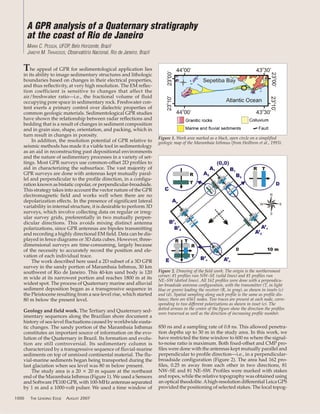
1. The appeal of GPR for sedimentological application lies
in its ability to image sedimentary structures and lithologic
boundaries based on changes in their electrical properties,
and thus reflectivity, at very high resolution. The EM reflec-
tion coefficient is sensitive to changes that affect the
air/freshwater ratio—i.e., the fractional volume of fluid
occupying pore space in sedimentary rock. Freshwater con-
tent exerts a primary control over dielectric properties of
common geologic materials. Sedimentological GPR studies
have shown the relationship between radar reflections and
bedding that is a result of changes in sediment composition
and in grain size, shape, orientation, and packing, which in
turn result in changes in porosity.
In addition, the resolution potential of GPR relative to
seismic methods has made it a viable tool in sedimentology
as an aid in reconstructing past depositional environments
and the nature of sedimentary processes in a variety of set-
tings. Most GPR surveys use common-offset 2D profiles to
aid in characterizing the subsurface. The vast majority of
GPR surveys are done with antennas kept mutually paral-
lel and perpendicular to the profile direction, in a configu-
ration known as bistatic copolar, or perpendicular-broadside.
This strategy takes into account the vector nature of the GPR
electromagnetic field and works well when there are no
depolarization effects. In the presence of significant lateral
variability in internal structure, it is desirable to perform 3D
surveys, which involve collecting data on regular or irreg-
ular survey grids, preferentially in two mutually perpen-
dicular directions. This avoids mixing distinct antenna
polarizations, since GPR antennas are bipoles transmitting
and recording a highly directional EM field. Data can be dis-
played in fence diagrams or 3D data cubes. However, three-
dimensional surveys are time-consuming, largely because
of the necessity to accurately record the position and ele-
vation of each individual trace.
The work described here used a 2D subset of a 3D GPR
survey in the sandy portion of Marambaia Isthmus, 30 km
southwest of Rio de Janeiro. This 40-km sand body is 120
m wide at its narrowest portion and reaches 1800 m at its
widest spot. The process of Quaternary marine and alluvial
sediment deposition began as a transgressive sequence in
the Pleistocene resulting from a sea-level rise, which started
80 m below the present level.
Geology and field work. The Tertiary and Quaternary sed-
imentary sequences along the Brazilian shore document a
history of sea-level fluctuations caused by worldwide eusta-
tic changes. The sandy portion of the Marambaia Isthmus
constitutes an important source of information on the evo-
lution of the Quaternary in Brazil. Its formation and evolu-
tion are still controversial. Its sedimentary column is
characterized by a transgressive sequence of fluvial-marine
sediments on top of unmixed continental material. The flu-
vial-marine sediments began being transported during the
last glaciation when sea level was 80 m below present.
The study area is a 20 ǂ 20 m square at the northeast
end of the Marambaia Isthmus (Figure 1). We used a Sensors
and Software PE100 GPR, with 100-MHz antennas separated
by 1 m and a 1000-volt pulser. We used a time window of
850 ns and a sampling rate of 0.8 ns. This allowed penetra-
tion depths up to 30 m in the study area. In this work, we
have restricted the time window to 600 ns where the signal-
to-noise ratio is maximum. Both fixed-offset and CMP pro-
files were done with the antennas kept mutually parallel and
perpendicular to profile direction—i.e., in a perpendicular-
broadside configuration (Figure 2). The area had 162 pro-
files, 0.25 m away from each other in two directions, 81
NW–SE and 81 NE–SW. Profiles were marked with stakes
and ropes, while the relative topography was obtained using
an optical theodolite.Ahigh-resolution differential Leica GPS
provided the positioning of selected stakes. The local topog-
A GPR analysis of a Quaternary stratigraphy
at the coast of Rio de Janeiro
MARIA C. PESSOA, UFOP, Belo Horizonte, Brazil
JANDYR M. TRAVASSOS, Observatório Nacional, Rio de Janeiro, Brazil
1000 THE LEADING EDGE AUGUST 2007
Figure 1. Work area marked as a black, open circle on a simplified
geologic map of the Marambaia Isthmus (from Heilbron et al., 1993).
Figure 2. Drawing of the field work. The origin is the northernmost
corner; 81 profiles run NW–SE (solid lines) and 81 profiles run
NE–SW (dotted lines). All 162 profiles were done with a perpendicu-
lar-broadside antenna configuration, with the transmitter (T, in light
blue or green) leading the receiver (R, in gray), as shown in insets (c)
and (d). Spatial sampling along each profile is the same as profile dis-
tance; there are 6561 nodes. Two traces are present at each node, corre-
sponding to two different polarizations as shown in inset (e). The
dotted arrows in the center of the figure show the direction the profiles
were traversed as well as the direction of increasing profile number.

2. raphy can be disregarded when compared to the vertical res-
olution of our survey.
Spatial sampling along each profile was variable, rang-
ing from 0.05 to 0.20 m subsequently decimated to a con-
stant step size of 0.25 m (equal to the distance between
profiles). In this way, we ended up with a grid of 6561 nodes,
each having two GPR traces obtained with two mutually
perpendicular copolar antenna configurations (Figure 2).
Processing included dewow, spatial and temporal filtering,
SEC (spreading and exponential compensation) gain, and
poststack migration along both directions. Both vertical and
horizontal resolution are conditioned by the spatial deci-
mation, the latter being greater than 0.25 m. Spatial filter-
ing was used to prevent alias on the decimated data set. The
attenuation coefficient used in the SEC gain was estimated
from the envelope exponential decay.
Results. The velocity spectra obtained from CMP gathers
implied a decreasing velocity model with depth for the
whole area: 0.13 m/ns (0–240 ns); 0.11 m/ns (240–280 ns)
and 0.09 m/ns (> 280 ns). This seems to be a bit too high as
a borehole adjacent to the survey area reveals wet sand at
3 m, or about 50 ns. This CMP-derived velocity model was
initially inappropriate for migrating our GPR sections. We
then used this model as a starting point in a trial-and-error
procedure to obtain a migration velocity model. A two-
velocity model yielded the best migrated image: 0.07 m/ns
(0–300 ns) and 0.05 m/ns onward. As a further simplifica-
tion, we adopted a single velocity model consisting of 0.06
m/ns, a value that seemed best suited for the saturated por-
tion of the subsurface. We used this model to migrate all
data using Kirchhoff poststack migration. We adopt the
median of all velocity estimates for depth conversion (0.09
m/ns).
The 81 NW–SE profiles cut the 81 NE–SW profiles at 6561
nodes where we have two traces obtained with perpendic-
ular-broadside antenna configurations in relation to the two
profile directions (Figure 2). In general, ties between per-
pendicular profiles were good, demonstrating the continu-
ity of reflectors across sections (Figure 3).
We can interpret our GPR sections in terms of radar
wavelet packages, depositional units consisting of geneti-
cally related strata, bounded by radar surfaces expressing
existing unconformities or the correlative conformities of the
unit. We will use the term facies when referring
to sets of reflections lying between radar surfaces.
We will assume here that we can apply the same
principles underlying seismic stratigraphy to our
radar data collected in a Quaternary sedimentary
environment. In this manner, radar surfaces, radar
packages, and radar facies are defined in the same
way as the equivalent terms in seismic stratigra-
phy for a given GPR reflection profile.
We interpret the sedimentary facies and facies
associations in a given NW–SE radar reflection
profile (S76 in Figure 3) to determine the deposi-
tional environment at the limit of GPR resolu-
tion. Profile S76 alone includes five radar facies
(Figure 4). Direct ground truth was not possible
because the loose sand near surface was not suit-
able for trenching. We label the observed radar
facies as A, B, A’, C, and D (Figure 5) and describe
them below.
Sheet packages A and A’ are characterized by
a planar reflection configuration with parallel and
continuous high-amplitude reflections. The lower
boundary onlaps on facies B. Facies A can be
related to a uniform deposition rate in a low energy envi-
ronment, typical of a beach strandplain or shore mud (Figure
5). Since penetration is good, we can assume deposition of
very fine sand grains and some clay.
Sigmoidal reflectors in facies B are characterized by a
curved reflection gently dipping to the southeast with mod-
erately continuous, oblique, high-amplitude reflections.
Reflections end in a downlap at the lower boundary evi-
denced by wavy reflections with good continuity. The top
boundary is truncated or ends as a toplap event at facies A.
The oblique reflection configuration of facies B indicates
moderate-to-high depositional energy with great volumes
of sediments moving in this area, suggesting this reflection
package is probably returning from a subparallel direction
in relation to profile S76 (Figure 5). Reflectors in facies B prob-
ably represent a sedimentation unit due to the transport of
shelf sediments toward the coast at the end of a marine trans-
gression. The overall geometry and internal structure of
facies B can be represented as a 3D cube (Figure 6). Note
that the reflection geometry reported here is consistent with
several different depositional scenarios found elsewhere in
coastal Brazil.
Sigmoidal reflections in sheet drape facies C are char-
AUGUST 2007 THE LEADING EDGE 1001
Figure 3. Two perpendicular GPR profiles shown in a fence diagram. Profile S76
runs NE–SW, and E29 runs NW–SE.
Figure 4. GPR section of reflection profile S76, which cuts the work
area NE–SW. This profile allows identification of five radar facies.

3. acterized by a curved reflection dipping to the southeast with
continuous subparallel medium-amplitude reflections. There
is a conspicuous mix of oblique and tangential reflections
in the section. The observed good penetration of the GPR
signals associated with the degree of saturation observed in
the borehole suggests very low clay and silt content through
the section. This facies is probably related to the eolian depo-
sition that occurred in this area (Figure 5). This interpreta-
tion is corroborated by the fact that sigmoidal reflectors
appear oriented along blowouts and by shallow (~5 m) drill
holes not far from a study area that reported a granulometric
transition from medium-to-finer sand from 3 m downward.
This lower horizon is characterized by well selected
reworked round sand grains.
Results suggest an increase in transgression rates fol-
lowing lower sea levels that pushed marine sediments on
top of fluvial deposits, facies A and B. We speculate one sea
level rise may correspond to the transgression that occurred
circa 3 Ma. Dunes may have formed during the period of
lower sea levels filling up topographic lows, consistent with
the oblique reflectors present in the section, facies C.
Conclusions. The results demonstrate that GPR can image
structures within unconsolidated sediments in the study
area sufficiently to allow data interpretation using the prin-
ciples of radar stratigraphy. We have used a single profile
to describe and interpret five radar facies. Supplementary
geologic information, ground truthing, and laboratory data
can be used with radar stratigraphy to produce a full sedi-
mentological interpretation. Judicious data processing pro-
vided an accurate record of the subsurface location and
orientation of reflections caused by the primary sedimen-
tary structure. A 3D analysis may prove useful in eliminat-
ing artifacts arising from lateral variability in internal
structure of the sediments. In this case results may best be
presented as 3D data cubes.
Suggested reading. “Three-dimensional multicomponent geo-
radar imaging of sedimentary structures” by Streich et al. (Near-
Surface Geophysics, 2006). “Ground-penetrating radar and its use
in sedimentology: Principles, problems and progress” by Neal
(Earth-Science Reviews, 2004). Ground-Penetrating Radar in
Sediments, edited by Bristow and Jol (Geological Society of
London, 2003). “Late Quaternary stratigraphy and sea-level
history of the northern Delaware Bay margin, southern New
Jersey, USA: A ground-penetrating radar analysis of compos-
ite Quaternary coastal terraces” by O’Neal and McGeary
(Quarterly Science Review, 2002). “Response of ground-pene-
trating radar to bounding surfaces and lithofacies variations in
sand barrier sequences” by Baker (Exploration Geophysics, 1991).
“Dina˘mica sedimentar da Restinga de Marambaia e Baía de
Sepetiba (Sedimentary dinamics of the Marambaia Isthmus
and Sepetiba Bay)” by Borges (master’s thesis, Federal
University of Rio de Janeiro, 1990). “Ground-penetrating radar
for high-resolution mapping of soil and rock stratigraphy” by
Davis and Annan (Geophysical Prospecting, 1989). “Sobre a
origem da Restinga de Marambaia (On the origin of the
Marambaia Isthmus, in Portuguese)” by Ponçano et al.
(Simpósio Regional de Geologia, 2, Rio Claro. Atas, Rio Claro,
SP, Volume 1, 1979). “Compartimentaça˜ tectoˆnica e evoluça˜o
geológica do segmento central da Faixa Ribeira, a sul do Cráton
do Sa˜o Francisco (Tectonics and geologic evolution of the cen-
tral portion of the Ribeira Belt, South of San Francisco Craton,
in Portuguese)” by Heilbron et al. (in Anais do II Simpósio sobre
o Cráton do Sa˜o Francisco, Salvador, SBG, 1993). TLE
Corresponding author: jandyr@on.br
1002 THE LEADING EDGE AUGUST 2007
Figure 5. Interpretation of the five sedimentary facies (labeled A, B, A’,
C, and D) identified in profile S76.
Figure 6. 3D view of the sigmoidal reflectors of facies B showing a
conspicuous increase in volume of shelf sediments from south to north
that occurred at the end of a marine transgression. The yellow arrow
shows the inferred average depositional direction toward the end of the
transgression. The dashed lines mark the limits between different depo-
sitional sequences.