This project was developed for an Embedded systems class: we implemented a PID controller for a mechanical inverted pendulum. It was very interesting to experiment in practice with a simple control plant.

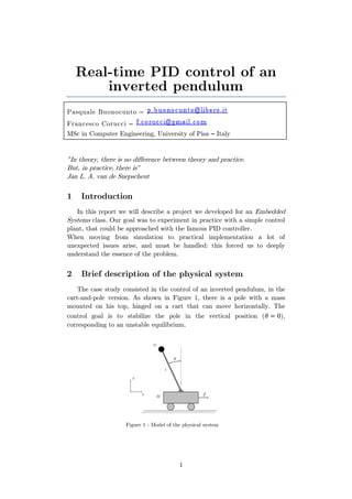
1. 1
Real-time PID control of an
inverted pendulum
Pasquale Buonocunto –
Francesco Corucci –
MSc in Computer Engineering, University of Pisa – Italy
"In theory, there is no difference between theory and practice.
But, in practice, there is"
Jan L. A. van de Snepscheut
1 Introduction
In this report we will describe a project we developed for an Embedded
Systems class. Our goal was to experiment in practice with a simple control
plant, that could be approached with the famous PID controller.
When moving from simulation to practical implementation a lot of
unexpected issues arise, and must be handled: this forced us to deeply
understand the essence of the problem.
2 Brief description of the physical system
The case study consisted in the control of an inverted pendulum, in the
cart-and-pole version. As shown in Figure 1, there is a pole with a mass
mounted on his top, hinged on a cart that can move horizontally. The
control goal is to stabilize the pole in the vertical position ( ),
corresponding to an unstable equilibrium.
Figure 1 - Model of the physical system

2. 2
3 Testbed
3.1 Plant
Figure 2 shows the real plant on which we worked. The cart is actuated
with a DC motor through a belt: the motor also provides an encoder, that
we used to deduce the horizontal position of the cart. The inclination of the
pole is measured with a potentiometer placed at its bottom.
Figure 2 – The plant
The motor (Figure 3) is a ESCAP DC
MOTOR/ENCODER 22V E9-0500-2.0-1: it
is a little bit underutilized since the board
Belt
Potentiometer
DC Motor
Motor encoder
Figure 3 - The DC motor used to control
the plant

3. 3
provides it less voltage/current than expected, but we used it anyway since
we had just demonstration purposes (otherwise a dedicated power circuit
should have been necessary). Other limitations of the plant will be
discussed later in this paper.
3.2 Control electronics
Figure 4 shows the control electronics.
Figure 4 - Control electronics
We used an Evidence1
FLEX motion board equipped with the DC
Motor plug-in. The board mounts a microcontroller of the dsPIC33 serie.
We also realized a simple circuit with three potentiometers, in order to be
able to regulate online the control parameters. The wiring is realized as
follows (refer to the appendix for the nomenclature):
1
http://www.evidence.eu.com
CON23
PIN NO. 4 3 2 1
CONNECTED TO B A + -
CON22
PIN NO. 2
CONNECTED TO ENC_STDBY
CON24
PIN NO. 4 3
CONNECTED TO Vmotor+ Vmotor-

4. 4
CON8
PIN NO. 20 19 12 10 2 1
CONNECTED
TO
- + Ki_POT Kd_POT POLE_POT Kp_POT
DC Motor + encoder
B, A, +, -
Vmotor+, Vmotor-
ENC_STDBY
EncoderDC motor
Kp Ki Kd
+
Bar
potentiometer
-
Figure 5 - Wiring scheme

5. 5
4 Angle control: the first PID controller
For what concerns the stabilization of the pole, we implemented a speed
control of the DC motor using a PID controller.
Below the digital implementation of the PID controller (simplified code):
float PID(float setpoint,float actual_position)
{
static float pre_error = 0.0;
static float integral = 0.0;
static EE_UINT8 count = 0;
static float errors[I_WINDOW_SIZE];
float error;
float derivative;
float output;
EE_UINT8 i;
...
// Calculate error
error = setpoint - actual_position;
// Integral component
if(Ki > 0.0 && WINDOWED_INTEGR)
{ // Windowed integration mode
integral = 0.0;
// The truncated integration is realized with
// a cyclic array
// Insert new value in the window
errors[count] = error;
// Update counter
count = (count+1) % I_WINDOW_SIZE;
// Accumulation
for(i = 0; i < I_WINDOW_SIZE; i++)
integral += errors[i]*dt;
}
else if(Ki > 0.0) // Non-windowed integration mode
integral += error*dt;
//
// Anti-windup saturation of integral component
//
float Ki_integral = Ki*integral;
if(Ki_integral> ANTI_WINDUP_THR)
Ki_integral = ANTI_WINDUP_THR;

6. 6
else if(Ki_integral < -ANTI_WINDUP_THR)
Ki_integral = -ANTI_WINDUP_THR;
// Derivative component
derivative = (error - pre_error)/dt;
// Calculate output
output = Kp*error + Ki_integral + Kd*derivative;
...
//Saturation Filter
if(output > MAX_PID)
{
output = MAX_PID;
}
else if(output < MIN_PID)
{
output = MIN_PID;
}
//Update error
pre_error = error;
return output;
}
Figure 6 - Digital implementation of the PID controller
Some comments about the code:
- It is possible to choose two different modes of integration: windowed
and not windowed
- Our PID provides an anti-windup saturation of the integral component
- The control output is (obviously) saturated
5 Position control: the second PID
A PID is sufficient to stabilize the pole in a vertical position, but since
the rail is bounded it is important to make the controller aware of the fact
that it could end up hitting the physical bounds of the rail (this is possible
in practice using an encoder placed on the DC motor, whose angular
information is translated into a linear one). A software strategy that tries
to manually manage this condition preserving the stability of the pole is
quite difficult to think. We thought that the better thing to do was to try
to keep the cart away from the bounds (ideally in the center of the rail)

7. 7
with some additional control, in order to decrease the probability of hitting
the bounds.
Theoretically speaking it should be necessary a much more complex
modellization in order to simultaneously control the angle of the pole and
the position of the cart, since the two variables are not independent.
However, trying to keep things easy, we tried an alternative way to realize
something similar to the ideal behavior. We programmed two independent
PID controllers, one for the angle stabilization, one for the position
stabilization, and we tuned the parameters in order to give more priority to
the angle stabilization: this way we are able to obtain a quite stable system,
that tries to converge to the center of the rail when this does not disturb
the pole stabilization. This corresponds to a simplification of the model,
that can be mitigated with an appropriate tuning of the parameters2
. We
like to think this simplified modellization as if the second PID (the position
control) acts like a disturbance on the first PID (the angle stabilization
controller). Figure 7 shows the block description of the system.
The code below illustrates how this was implemented (pseudocode):
float current_position = <get pole inclination>;
float current_ticks = <get cart displacement from center>;
float angle_control = PID1(ANGLE_SETPOINT,
current_position);
float position_control = PID2(POSITION_SETPOINT,
current_ticks);
float control = angle_control + position_control;
<saturation of the resulting control variable>
Figure 8 - Control variable calculation
2
This is the interpretation we gave to our idea, that seems to be confirmed by
some works found in literature, like [1]
Ref
angle
PID1
PID2
Ref
pos
+ PLANT
+
-
+
-
pole_angle
cart_position
angle_control
pos_control
control
Figure 7 - Complete control system

8. 8
For what concerns the output control variable (controlling the speed of the
DC motor), it was saturated from -100 to +100, using the sign as
discriminator for the direction. The amplitude is from 0 to 100 because the
control is a PWM duty creating a linear voltage for the DC motor.
However, due to practical limitations caused by the cart friction on the rail,
the minimum PWM duty cycle usefull to really move the cart is quite high
(about 30% with good lubrification), so we limitated it in a shorter range
defined by two thresholds (±[MIN_PID, MAX_PID]).
6 PID tuning
Given the control system architecture, the proper way to tune the whole
system is the following:
1. Keeping the second PID disabled, tune the parameters of the first
PID (the angle stabilization one) as if it is the only controller in the
system;
2. Once the angle stability is reached, enable and tune the second PID
(the position control one) with “light” parameters, in order to preserve
the angle stabilization previously obtained.
The single PID can be tuned with any of the classical methods, such
Ziegler-Nichols: we followed an heuristic methodology inspired to the latter,
also driven by the practical interpretation we gave to every parameter.
7 Software organization
The application is composed of 5 tasks:
- TASK_HOMING [aperiodic]: activated only one time at the startup, it
manages the necessary homing steps in order to make system aware of
the control set points (rail center, and pole equilibrium position). It
requires the user intervention.
- TASK_POSITION_CONTROL [period: 150ms, priority: 53
]: reads the
position of the cart and calculates the PID for the position control. The
computed value is used from the the angle control task, that performs
the real actuation merging the two control variables.
- TASK_ANGLE_CONTROL [period: 50ms, priority: 6]: reads the
inclination of the bar, calculates the PID for the stabilization of the
bar, combines this value with the one from the position control task,
then actuates the motor.
3
Task priority in OSEK is specified by a number from 1 to 10. Higher values
represents higher priorities

9. 9
- TASK_READ_POT [period: 200ms, priority: 3]: this task acquires
values from the three external potentiometer, and updates the control
parameters accordingly.
- TASK_SERIAL_PRINT [period: 500ms, priority: 2]: feedsback some
useful information via UART.
Figure 9 shows the execution flow of the application:
8 Running demonstration
A running demonstration of the implemented system can be viewed in the
following videos:
http://www.youtube.com/watch?v=zEF6a_m0kdQ
http://www.youtube.com/watch?v=9Mg-y6TDef4
9 Limitations
The physical system we worked on presented considerable non-idealities,
that made quite hard the task of making things work properly. The main
limitation of the plant relies in the friction between the rail and the cart,
that remains considerable also with appropriate lubrification. Also the
traction offered by the belt is asymmetric in the two direction and causes
some extra friction. Another issue relies in the motor, its poor precision and
its underutilization (since the board provides it less voltage/current than
1. Maintain the bar, press the
button, and let the cart
scan the rail to identify the
center
2. Once the cart have reached
the center of the rail, put
the pole in the steady state
and press again the button
main init
TASK_HOMING
button pressed / activate task
TASK_POSITION_
CONTROL
TASK_ANGLE_
CONTROL
button pressed / activate task
TASK_SERIAL_
PRINT
TASK_READ_
POT
Figure 9 - Execution flow

10. 10
expected). The final effect of these limitation is that the movements of the
cart are inevitably jerky, making quite difficult to obtain a smooth control
and, as a consequence, a good stabilization of the system.
10 Future work
The potentiometer used to read the inclination of the pole is quite noisy:
with a rough strategy, we just truncated the measures after the second
decimal digit, because all we got beyond that was nothing but noise. This
was enough for our purposes, but it should be interesting, instead, to
implement some filtering strategy to gain accuracy in the angle
measurement. For example it could be usefull to oversample the value with
a higher frequency in respect to the control frequency (i.e. the frequency
with which the measure is consumed), and then apply some filtering (es:
low pass, median, …). Another filter that is commonly used in this context
is the Kalman filter, used to estimate the measure ensuring a good
immunity to noise.
11 References
[1] “Simulation and Robustness Studies on an Inverted Pendulum”, HUANG
Chun-E, LI Dong-Hai, SU Yong, Proceedings of the 30th Chinese Control
Conference, July 22-24, 2011, Yantai, China

11. 11
12 Appendices

12. 12