Many network simulators (e.g., ns2) are already being used for performing wired and wireless network simulations. But, with the current graphical visualization support in-built in ns2, it is difficult to understand the node status, packet status and the MAC level events particularly for Ad-hoc networks. In this paper, we extend the visualization support in ns-2 that should help research community in the area of wireless networks to analyze different MAC level events in an efficient manner. In particular, we have developed two types of visualizations namely, temporal and spatial. Temporal visualization helps to analyze success or failure of a packet with respect to time while spatial visualization helps to understand the effects due to proximity of nodes. The trace is made highly configurable in terms of different attributes like specific nodes and time duration.

1. Regular Paper
Proc. of Int. Conf. on Advances in Recent Technologies in Communication and Computing
Graphical Visualization of MAC Traces for Wireless
Ad-hoc Networks Simulated in ns2
1
Manan Thakar, 2Yogendra Raulji, 3Jayrajsinh Gohil, 4Hardik Mistry,
5
Mayur M Vegad and 6Dr. Narendra M Patel
Gujarat Technological University, Ahmedabad, Gujarat, India
1
manan_thakar@yahoo.co.in, 2raulji.yogendra@gmail.com, 3jaygohil1710@gmail.com, 4hardikmistry.1992@gmail.com
mayurmvegad, nmpatel@bvmengineering.ac.in
Abstract - Many network simulators (e.g., ns2) are already
being used for performing wired and wireless network
simulations. But, with the current graphical visualization
support in-built in ns2, it is difficult to understand the node
status, packet status and the MAC level events particularly
for Ad-hoc networks. In this paper, we extend the visualization
support in ns-2 that should help research community in the
area of wireless networks to analyze different MAC level
events in an efficient manner. In particular, we have developed
two types of visualizations namely, temporal and spatial.
Temporal visualization helps to analyze success or failure of
a packet with respect to time while spatial visualization helps
to understand the effects due to proximity of nodes. The trace
is made highly configurable in terms of different attributes
like specific nodes and time duration.
A. Input from users
Usually, there would be many nodes and many activities
and events in the network at runtime. But, we will have to
know the particular nodes for which the user wants to see
the visualization.
So, the inputs required from the user are:
1) Number of nodes for which the visualization is
needed.
2) Particular node numbers for which the visualization
is needed.
3) The time period for which the visualization is
needed.
Thus, the nodes for which the visualization is needed
and for which time period is needed, is acquired by the dialogbox
Index terms- Network event tracing, wireless networks, network
simulator, MAC layer, graphical visualization, ns2, collision,
packet, topography
B. Trace File
All the details about the packet and the events will be
acquired from the trace file of ns2. Here, trace file is a file
containing the traces of various events at different layers,
generated by the simulator ns2. When the TCL script describing the network scenario is run on ns2, the trace file is
created having the information about the events in network.
From this trace file, we can get the following information:
Event type (sent, received, dropped, forward), time instant,
node number (node-id), trace name (at which layer the event
occurred), reason (collision, retry-limit-reached, etc), event
identification number (event-id), packet type (RTS, CTS, tcp,
etc), size of the packet, duration field of MAC frame, (MAC
level) destination , (MAC level) source, type (ARP – 0x0860
/ IP – 0x0800).
This file is read by our program and the useful attributes
to build the visualization are stored in the data structure.
Here, to store such attribute=s, we have used appropriate
java-classes. Such classes are described in the next section.
I. INTRODUCTION
A network simulator is a tool for implementing the network on the computer. With the help of a simulator, the
behaviour of the network is calculated either by network entities interconnection using mathematical formulas, or by
capturing and playing back observations from the simulated
network. Network simulators like ns2, ns3, OPNET, NetSim,
OMNeT++, REAL, J-Sim and QualNet are already being used
for performing wired and wireless network simulations. But it
is difficult to understand the status of the nodes & packets
and the MAC level events particularly for Ad-hoc networks.
The resulting product of this work is useful to visualize and
analyze the different MAC level events for ad hoc wireless
networks when simulated in ns2. In this paper, we emphasize
on the main features of events and packets and provide a
comprehensible visualization for them. It is hoped that, this
work will prove to be a good reference source for those people
who feel difficult to analyze the MAC level events for wireless Ad-hoc networks.
C. Node-position-scenario File
This is (usually, a separate) text file in TCL, specifying
the positions (in Cartesian coordinates) of the participating
nodes. This information is used to determine the network
topology and is read by the main TCL script as an input.
Moreover, if the nodes are moving from one place to other
place, than such movements are also specified in this file.
Thus, the scenario file specifies:
1)
The co-ordinates of nodes
2)
Movements of nodes
II. SYSTEM INPUTS
For creating visualization, information about the nodes,
events and packets of the network is required. For that, we
take some inputs from various sources.
© 2013 ACEEE
DOI: 03.LSCS.2013.5. 548
53

2. Regular Paper
Proc. of Int. Conf. on Advances in Recent Technologies in Communication and Computing
packet is also calculated using the received power. The width
will be proportional to the size of the packet. Then, the packet
is drawn at the particular time on the graph Then, the packet
is drawn with green color if distance is within the transmission range. If distance is greater than transmission range but
within the threshold range, then fill it with yellow packet.
For detecting the collision, for each packet, the
interference range of the receiver is found. For finding
interference range, the below formula is considered
Interference range =(δ1/α ) *distance, Where δ = Capture
Threshold (minimum signal-to-interference ratio for
successful reception) with default value of 10, α = path-loss
factor (with default value of 4) distance = distance between
sender and receiver. Now, for this receiver, check whether
any other node within the interference range is trying to send
a packet during same time or not. If such packet is found,
then it will be dropped. So, draw it with RED color. Define the
mouse clicking event. Here, on clicking any packet, the packet
details should be displayed. For the collided packet, it is
collided with which packet is also specified.
It is worth noted here that, for detecting a collision, we
have calculated the interference range and based on that, the
collision is detected. Though, such information about a
collision event is already available in the trace file in ns2, in
the following we explain why it was required to calculate the
interference range.
III. IMPLEMENTATION
We have used java programming for the implementation.
Particularly, the java-graphics objects are used for graphical
presentation and swing properties of java are also used along
with them.
Now the implementation for temporal and spatial visualization is explained.
A. Implementation of Temporal Visualization
After achieving the input information, that information is
plotted on the graph to make visualization. This algorithm is
for visualization-1.
The algorithm to plot the visualization graph is as below:
The axis for the graph is drawn for each node. (X-axis specifies the time and y-axis specifies the power of transmission
or reception.)Set start-time specified by user as the starting
time in the graph.
For sending packet, the rectangle is drawn on the appropriate sender node graph. The height of this rectangle is the
maximum unit strength) as the power of sending packet is the
maximum and the width will be proportional to the size of the
packet. Fill it with BLUE color for the send packet.
For each node other than sender node for a particular
event, the distance of the node from the sender node is calculated. If this distance is in the threshold range, then the
power of the received packet is calculated. The height of the
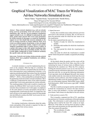
Fig. 1 Graphical Visualization
B. Implementation of Spatial Visualization
If the visualization2 (spatial visualization) is selected
after taking input, the following steps are carried out:
1) The nodes are drawn at their position specified in the
scenario file with their threshold range and transmission range.
Here, threshold range is specified in the blue color and the
transmission range is drawn in black color.
In the trace file, the ending time of the collided packet is
specified and not the beginning time of collision. Moreover,
we cannot determine with which packet a particular packet is
collided. For solving these problems, we have used the
interference range and based on that, the collision event is
traced and the packet causing the collision is determined
easily.
© 2013 ACEEE
DOI: 03.LSCS.2013.5. 548
54

3. Regular Paper
Proc. of Int. Conf. on Advances in Recent Technologies in Communication and Computing
Fig. 2 Graphical Visualization showing details of packet
Fig. 3 Spatial Visualization
2)The time-bar is drawn at bottom of the nodal
representation. One marker is shown moving with the time to
reflect the current time.
3) With the time, interference range is drawn at the
reception node of the packet. Interference range is drawn
with red color.
4) With the progression in transmission time of a given
packet, the packet is shown moving from source to destination
© 2013 ACEEE
DOI: 03.LSCS.2013.5. 548
. A successfully received packet is drawn with blue color,
whereas a collided packet is drawn with red color.
By implementing this algorithm, the spatial visualization
is generated.
IV. VISUALIZATION
A. Temporal Visualization
This figure shows details of 4 nodes as sender and
55

4. Regular Paper
Proc. of Int. Conf. on Advances in Recent Technologies in Communication and Computing
receiver side on time scale.
Here, the following points are to be noted:
A blue colored packet is a sent packet and a green packet
is a received packet.
Width of packet in graph is proportional to the actual size
of the packet. For example, the width of a data packet is
(usually) larger than the width of RTS/CTS packet as
observed in Fig. 1.
 A yellow packet shows that the corresponding receiving
node is in the carrier sensing range of the corresponding source node. This indicates that this particular packet
is a ‘sensed only’ (i.e., non-decodable) kind of packet.
In other words, such a transmission is sensed but the
packet cannot be interpreted.
The height of the packet in graph is proportional to the
transmitted or received power of the packet. Here, it can
be observed that the height of green packet (receiving)
is less than that of blue (sending) packet as obvious.
 A red packet shows the dropped packets. One of the
reasons for dropping could be a collision with some
other packet.
As the wireless link is of broadcast nature, a packet is
received by all the nodes within the transmission range of the
sender
When a particular packet, (sent or received) is clicked
with a mouse, its details are displayed as shown in Fig. 2.
Here, all the details of the clicked packet are shown as the
message. A click on OK button gets dialog-box disappeared.
In Fig. 2, the details of a collided packet are shown. Here, it
can be observed that the details of both the packets which
are collided are displayed.
For this scenario, the data-packet sent by node 0 destined
to node 1 is sensed by node 2. Now during that time, node 3
(a hidden terminal) also starts to send a packet to node 2. This
results into a collision at node 2. This is clearly depicted in
Fig. 2.
The description of each of the range is as follows:
1. Carrier sense range: in which, the packet is sensed.
2. Transmission range: in which, the packet is
successfully received (decodable).
3. Interference range: within which, if some other node
transmits concurrently then collision happens.
Thus, in spatial visualization, topography of each node
is displayed. In the specific example depicted in Fig. 3, it can
be observed that, node 0 is transmitting a packet to node 1.
Now at the same time, node 3 also tries to send packet to
node 2. As seen, node 2 is also in the interference range of
node 1. Consequently, the packets are collided.
V. CONCLUSION
Current graphical visualization support in ns2 lacks the
details of MAC level event traces like collisions. In this work,
we have attempted to mitigate this limitation. Two types of
graphical visualization are offered: temporal and spatial.
The temporal view of packets incorporates the details of
collision and overlapping of packets with respect to the
progression of simulation time. The spatial view incorporates
the physical activities happening at the nodes emphasizing
the effects of proximity of the participating nodes in space. It
is hoped that, this work would be extremely helpful to research
community in the area of wireless networks. It can be extended
also for further versions of ns2 and ns3.
REFERENCES
[1] Manual of ns2,available at http://www.sop.inria.fr/maestro/
personnel/Giovanni.Neglia/nscourse/ns course.htm.
[2] AT&T reference manual, Wireless personal communication,
1990.
[3] A. Tanenbaum, Computer Networks,4th edition, ch-4;.
[4] Introduction to Glomosim, available at http://
www.slideshare.net/ayyakathir/glomosim-introduction6476014.
[5] Introduction to Omnetpp, available at http://www.omnetpp.org/
pmwiki/ index.php?n=Main.OmnetppInNutshell.
[6] András Varga, Rudolf Hornig, An Overview of the OMNet++
Simulation Environment, SIMUTools, March03-07,2008,
Marseille, France.
[7] Dennis McGrath, Doug Hill, Amy Hunt, Mark Ryan, and
TimothySmith, NETSIM:A Distributed Network Simulation
to Support Cyber Exercises, Award No. 2000-DT-CX-K001
from the Office for Domestic Preparedness, U.S. Department
of Homeland Security
[8] Introduction to netsim, available at http://www.boson.com/
files/support/NetSim8LabCompiler.pdf.
[9] Marc Greis’ Tutorial for the UCB/LBNL/VINT Network
Simulator “ns”, available at http://www.isi.edu//tutorial
B. Spatial Visualization
One another type of visualization is – spatial visualization,
which shows the relative position of the nodes as per their
physical coordinates. This visualization also depicts different
nodal ranges around each of the selected nodes. A typical
sample output for spatial visualization is shown in Fig. 3.
It can be observed that, there are 4 nodes in this scenario.
The nodes are drawn on their coordinate positions as per
their relative positions. For this particular scenario, the nodes
are on a common horizontal line. The colored circles around a
particular node represent the ranges of that node. Particularly, the black circle around node shows its transmission
range, the blue circle shows its threshold range, and the red
circle shows its interference range (applicable to a receiver
node). At the bottom of Fig. 3, time-scale is displayed. As time
progresses, a vertical pointer moves towards right along with
x-axis. A particular instant of time is displayed above this time
scale. Numbers 0,1,2,3, etc show node positions according to
their coordinates.
© 2013 ACEEE
DOI: 03.LSCS.2013.5. 548
56