SlideShare uma empresa Scribd logo
1 de 36
Lecture Series on
  Biostatistics
                 No. Bio-Stat_3
                Date – 03.08.2008


     CLASSIFICATION
          AND
   TABULATION OF DATA
         Dr. Bijaya Bhusan Nanda,
     M. Sc (Gold Medalist) Ph. D. (Stat.)
    Topper Orissa Statistics & Economics
               Services, 1988
         bijayabnanda@yahoo.com
LEARNING OBJECTIVES
   The trainees will be able to do
    meaningful classification of large
    mass of data and interpret the same.

   They will be able to construct
    frequency distribution table and
    interpret the same.

   They will be able to describe different
    parts of tables and types of table
CONTENT
 Concept of Variable
 Ordered array
 What is data Classification ?
 Objectives of Classification
 Frequency distributions
   Variables and attributes
 Tabulation of data
   Parts of a table
   Type of tables
Concept of Variable
   Variable
    A characteristic which takes on different
    values in different persons, place or
    things.

    Example: Diastolic/Systolic blood
    pressure, heart rate, the heights of adult
    males, the weights of preschool children
    and the ages of patients seen in a dental
    clinic
   Quantitative Variable:- One that can be
    measured and expressed numerically. The
    measurements convey information regarding
    amount.
    Example: Diastolic/Systolic blood pressure, heart
    rate, the heights of adult males, the weights of
    preschool children and the ages of patients seen
    in a dental clinic

   Qualitative Variable:- The characteristics that
    can’t be measured quantitatively but can be
    categorized. The measurement convey
    information regarding the attribute. The
    measurement in real sense can’t be achieved but
    persons, places or things belonging to different
    categories can be counted.
    Example: sex of a patient, colure and odour of
    stool and urine samples etc.
Random Variable
   Values obtained arise as a result of chance
    event/factor, so that can’t be exactly predicted
    in advance.
    Example: heights of a group of randomly
    selected adult.
   Discrete Random Variable:- Characterized by
    gaps or interrupts in the values that it can
    assume.
        It assumes values with definite jumps.
        It can’t take all possible values within a
    range.
        It is observed through counting only
    Example: No. of daily admission to a general
    hospital, the no. of decayed, missing or filled
    teeth per child in an elementary school.
   Continuous Random Variable:-
     • It can take all possible values positive,
       negative, integral and fractional values
       within a specified relevant interval.
     • Doesn’t possess the gaps or
       interruptions within a specified relevant
       interval of values assumed by the
       variable.
     • Derived through measurement
    Example: height, weight and skull
    circumference
    Because of limitations of available
    measuring instruments, however
    observations on variables that are
    inherently continuous are recorded as if
    they are discrete.
The ordered array
   A first step in organizing data is
    preparation of an ordered array.
   It is a listing of values of a data series
    from the smallest to the largest values.
   It enables one to quickly determine the
    smallest and largest value in the data set
    and other facts about the arrayed data
    that might be needed in a hurried manner.
   Look at the unordered and ordered data in
    the file DataExample.xls
   DATA CLASSIFICATION: The grouping of
    related facts/data into different
    classes according to certain common
    characteristic.
        Basis of data Classification:
         • Broadly 4 broad basis
    1.     Geographical      i.e. area wise
             • Total Population of Orissa by
               districts
             • No. of death due to malaria by
               districts.
             • Infant deaths in Orissa by districts
2.   Chronological or Temporal
     •  i.e. on the basis of time
        Table: 2 Death by lightening

          Year     Number
           1990       10
           1991        5
           1992       12
           1993        6
           1994        9
           1995        3
           1996        3
           1997        5
           1998       12
           1999       12
           2000        8
           2001        7
           2002        8
           Total     100
3.    Qualitative i.e. on the basis of some
      attributes
      Example: People by place of residence, sex
      and literacy
                  Place of residence
                     Rural                                            Urban
           Male                  Female                    Male                   Female
     Literate   Illiterate   Literate   Illiterate   Literat   Illiterate   Literate   Illiterate
                                                     e
4.   Quantitative: On the basis of
     quantitative class intervals

 For example students of a college may be classified
 according to weight as follows
         Table 3 :Weight of students of a college
         Wt. In (LBS) No. of students

            90-100             50
           100-110            200
           110-120            260
           120-130            360
           130-140             90
           140-150             40
             Total           1000
Classification of Age of 600 person in
the Social Survey
  Class                      Relative
 Interval   Frequency       frequency
15 -24               56             09.3
25-34               153             25.5
35-44               149             24.8
45-54                75             12.5
55 - 64              61             10.2
65 - 74              70             11.7
75 - 84              28              4.7
85 - 94                8             1.3
Total               600            100.0
In a survey of 35 families in a village,
the number of children per family was recorded data were obtained.


       1         0         2        3      4      5        6
       7         2         3        4      0      2        5
       8         4         5        9      6      3        2
       7         6         5        3      3      7        8
       9         7         9        4      5      4        3
OBJECTIVES OF CLASSIFICATION
   Helps in condensing the mass of data
    such that similarities and dissimilarities can
    be readily distinguished.
      No. of        No of    Cum. Fre.  Cum.
     children      families  Less than  Fre.
                 (Frequency)           Greater
                                        than
        0-2           7          7       35
        3-5            16             23         28
      6 and            12             35         12
      above
       Total           35
   Facilitate comparison
     No. of        No of     Cum. Fre.    Cum.
    children     families    Less than    Fre.
               (Frequency)               Greater
                                          than
      0-2           7        7 (20%)    35
                                      (100)
      3-5          16           23      28
                             (65.7%) (80%)
    6 and          12           35      12
    above                    (100%) (34%)
     Total         35
   Most significant features of the data
    can be pin pointed at a glance
    Enables statistical treatment of the
    collected data
       Averages can be computed
       Variations can be revealed

       Association can be studied

       Model for prediction / forecasting can be

        built
       Hypothesis can be formulated and tested

        etc.
Principles of Classification:

There is no hard and fast rules for
 deciding the class interval,
 however it depends upon:
     Knowledge of the data
     Lowest and highest value of the

      set of observations
     Utility of the class intervals for

      meaningful comparison and
      interpretation
                   r
   The classes should be collectively
    exhaustive and non-overlapping i.e.
    mutually exclusive.

   The number of classes should not be too
    large other wise the purpose of class i.e.
    summarization of data will not be served.

   The number of classes should not be too
    small either, for this also may obscure the
    true nature of the distribution.

   The class should preferable of equal
    width. Other wise the class frequency
    would not be comparable, and the
    computation of statistical measures will
    be laborious.
   More specifically Struges formula can be used to
    decide the no. of class interval;
     • K=1+3.322(log 10n )
        Where k = no. of classes, n=no. of
       observation
   The width of the class interval may be
    determined by dividing the range by k
              w= R
                 k

    where R= difference between the highest and the
    lowest observation.
        w = width of the class interval
   When the nature of data make them appropriate
    class interval width of 5 units, 10 units and width
    that are multiple of 10 tend to make the
    summarization more comprehensible.
                             r
Classification will be called exclusive (Continuous),
when the class intervals are so fixed that the upper
limit of one class is the lower limit of the next class
and the upper limit is not included in the class.
 An example

              Income (Rs.)               No. of
                                        families
        1000 – 1100 = (1000 but under        15
        1100)
        1100 – 1200 = (1100 but under        25
        1200)
        1200 – 1300 = (1200 but under        10
        1300)
                     Total                  50
   Classification will be inclusive
    (discontinuous) when the upper and lower
    limit of one class is include in that class itself

           Income (Rs.)                 No. of
                                       persons
     1000 – 1099 = (1000 but <             50
     1099)
     1100 – 1199 = (1100 but <            100
     1199)
     1200 – 1299 = (1200 but <            200
     1299)
                 Total                    300
   Discontinuous class interval can be
    made continuous by applying the
    Correction factor.
           Lower limit of 2nd Class – Upper
                limit of the 1st Class
    CF =
                       2

    The correction factor is subtracted
    from the lower limit and added to
    the upper limit to make the class
    interval continuous.
Frequency distributions
   Quantitative Variables:
    •   Discrete variable
    •   Continuous variable
   Qualitative variable (attributes)

   The manner in which the total
    number of observations are
    distributed over different classes
    is called a frequency distribution.
Frequency distribution of an attribute
                           Table 4 : Results of survey
                          on Awarenesson HIV / AIDs
                          State of        Number of
   In 1993, 1674         Knowledge        people
    inhabitants of
                          Aware              620
    Calcutta, Bombay
                          Unaware            1054
    and Madras were
                          Total             1674
    surveyed. Each was
    asked, among,
    other questions,        Table 5 : Proportion of
                            people Aware of HIV /
    whether he/she                   AIDS
    knew about the HIV
                          State of        Relative
    / AIDS. The results
                          Knowledge      frequency
    is tabulated.
                             Aware         0.370
                            Unaware        0.630
                             Total         1.000
Frequency distribution of a discrete
                variable
   Data grouped in to classes and the number of
    cases which fall in each class are recorded

Example: In a survey of 35 families in a village, the number
of children per family was recorded data were obtained.

       1     0      2      3     4      5      6
       7     2      3      4     0      2      5
       8     4      5      9     6      3      2
       7     6      5      3     3      7      8
       9     7      9      4     5      4      3
Steps for frequency distribution
•   Find the largest & smallest value;
    those are 9 and 0 respectively.

•   Form a table with 10 classes for the
    10 values 0,1,2……9

•   Look at the given values of the
    variable one by one and for each value
    put a tally mark in the table against
    the appropriate class.

•   To facilitate counting, the tally marks
    are arranged in the blocks of five
    every fifth stroke being drawn across
    the proceeding four. This is done
    below.
Table 6: Frequency Table

                                Cumulative Cumulative
 No. of                         Frequency Frequency
         Tallies    Frequency
children                        Less than   More than
                                type          type
   0                  2           2          35
   1                   1           3          33
   2                4           7          32
   3                           13          28
                        6
           
   4                5          18          22
   5                5          23          17
   6                 3          26          12
   7                4          30          9
   8                  2          32          5
   9                 3          35          3
TABULATION OF DATA

   Compress the data into rows and columns
    and relation can be understood.

   Tabulation simplifies complex data,
    facilitate comparison, gives identify to the
    data and reveals pattern
Different parts of a table
   Table number
   Title of the table
   Caption: Column Heading
   Stub     : Row heading
   Body     : Contains data
   Head notes: Some thing that is not
    explained in the title, caption, stubs
    can be explained in the head notes on
    the top of the table below the title.
   Foot notes: Source of data, some
    exception in the data can be given in
    the foot notes.
Table can be classified into 3
           ways
   Type of table       Characteristic Feature
1. Simple table        only one characteristic is shown
2. Complex table

  a. Two way table    shows two characteristics and is
                      formed when either the stub or the
                      caption is divided in to two co-
                      ordinate parts
   b. Higher order    When three or more characteristic are
table                 represented in the same table, such a
                      table is called higher order table
3. General and        published by Govt. such as in the
special purpose table statistical Abstract of India, or census
                      reports are general purpose table
Complex table
  Average Number of OPD patients in a PHC in a
tribal area in different age group according of sex

                        OPD Patients
Age in yrs
                Male    Female      Total
 Below 25        25         5             30
   25-35         30         4             34
   35-45         25         5             30
  45-55          22         3             25
 Above 55        15         1             16
   Total        117        18            135
Number of patients in OPDs of Public sector
     hospital by Religion, Age, Rank and Sex
Religion Age(in yr.)                   Rank
                       Supervisor Assistant   Clerks   Total
                       F   M T    F M T       F M T    FMT
Hindu    Below 25
         25- 35
         35 – 45
         45 – 55
         55 & above
Muslim   Below 25
         25- 35
         35 – 45
         45 – 55
         55 & above
         Total
   Exercise
    Age of 169 subjects who
    participated in a study of
    Sparteine and Mephynytoin
    Oxidation is given. Calculate the
    frequency, cumulative frequency
    both less than and more than
    type, relative frequency and
    cumulative relative frequency.
    From these find out what is the
    proportion of patient aged 60 and
    more. (Data in the file
    DataExample.xls)
   Next Class:
    • Understanding data through
      presentations
THANK YOU

Mais conteúdo relacionado

Mais procurados

Measures of dispersion
Measures of dispersionMeasures of dispersion
Measures of dispersion
Sachin Shekde
 

Mais procurados (20)

Measures of central tendency and dispersion
Measures of central tendency and dispersionMeasures of central tendency and dispersion
Measures of central tendency and dispersion
 
Chi squared test
Chi squared testChi squared test
Chi squared test
 
Statistics
StatisticsStatistics
Statistics
 
#2 Classification and tabulation of data
#2 Classification and tabulation of data#2 Classification and tabulation of data
#2 Classification and tabulation of data
 
Tabular and Graphical Representation of Data
Tabular and Graphical Representation of Data Tabular and Graphical Representation of Data
Tabular and Graphical Representation of Data
 
Standard deviation
Standard deviationStandard deviation
Standard deviation
 
presentation of data
presentation of datapresentation of data
presentation of data
 
Test of significance in Statistics
Test of significance in StatisticsTest of significance in Statistics
Test of significance in Statistics
 
Diagrammatic and Graphical Representation of Data in Statistics
Diagrammatic and Graphical Representation of Data in StatisticsDiagrammatic and Graphical Representation of Data in Statistics
Diagrammatic and Graphical Representation of Data in Statistics
 
Measures of Central Tendency - Biostatstics
Measures of Central Tendency - BiostatsticsMeasures of Central Tendency - Biostatstics
Measures of Central Tendency - Biostatstics
 
sampling ppt
sampling pptsampling ppt
sampling ppt
 
Parametric vs Non-Parametric
Parametric vs Non-ParametricParametric vs Non-Parametric
Parametric vs Non-Parametric
 
Measures of dispersion
Measures of dispersionMeasures of dispersion
Measures of dispersion
 
Nature, Scope, Functions and Limitations of Statistics
Nature, Scope, Functions and Limitations of StatisticsNature, Scope, Functions and Limitations of Statistics
Nature, Scope, Functions and Limitations of Statistics
 
Meaning of statistics
Meaning of statisticsMeaning of statistics
Meaning of statistics
 
mean median mode
 mean median mode mean median mode
mean median mode
 
Correlation ppt...
Correlation ppt...Correlation ppt...
Correlation ppt...
 
Measures of dispersion
Measures of dispersionMeasures of dispersion
Measures of dispersion
 
Classification of data
Classification of dataClassification of data
Classification of data
 
Sampling
SamplingSampling
Sampling
 

Semelhante a Classification & tabulation of data

Tabulation of Data, Frequency Distribution, Contingency table
Tabulation of Data, Frequency Distribution, Contingency tableTabulation of Data, Frequency Distribution, Contingency table
Tabulation of Data, Frequency Distribution, Contingency table
Jagdish Powar
 
Presentation of data
Presentation of dataPresentation of data
Presentation of data
maryamijaz49
 
2. week 2 data presentation and organization
2. week 2 data presentation and organization2. week 2 data presentation and organization
2. week 2 data presentation and organization
renz50
 
Statics for management
Statics for managementStatics for management
Statics for management
parth06
 
Classidication and Tabulation
Classidication and TabulationClassidication and Tabulation
Classidication and Tabulation
Osama Zahid
 

Semelhante a Classification & tabulation of data (20)

Medical Statistics Part-I:Descriptive statistics
Medical Statistics Part-I:Descriptive statisticsMedical Statistics Part-I:Descriptive statistics
Medical Statistics Part-I:Descriptive statistics
 
Principlles of statistics [amar mamusta amir]
Principlles of statistics [amar mamusta amir]Principlles of statistics [amar mamusta amir]
Principlles of statistics [amar mamusta amir]
 
Fundamental of Biostatics DR.SOMANATH.ppt
Fundamental of Biostatics DR.SOMANATH.pptFundamental of Biostatics DR.SOMANATH.ppt
Fundamental of Biostatics DR.SOMANATH.ppt
 
1) Chapter#02 Presentation of Data.ppt
1) Chapter#02 Presentation of Data.ppt1) Chapter#02 Presentation of Data.ppt
1) Chapter#02 Presentation of Data.ppt
 
Tabulation of Data, Frequency Distribution, Contingency table
Tabulation of Data, Frequency Distribution, Contingency tableTabulation of Data, Frequency Distribution, Contingency table
Tabulation of Data, Frequency Distribution, Contingency table
 
Class1.ppt
Class1.pptClass1.ppt
Class1.ppt
 
Class1.ppt
Class1.pptClass1.ppt
Class1.ppt
 
Class1.ppt
Class1.pptClass1.ppt
Class1.ppt
 
Class1.ppt
Class1.pptClass1.ppt
Class1.ppt
 
STATISTICS BASICS INCLUDING DESCRIPTIVE STATISTICS
STATISTICS BASICS INCLUDING DESCRIPTIVE STATISTICSSTATISTICS BASICS INCLUDING DESCRIPTIVE STATISTICS
STATISTICS BASICS INCLUDING DESCRIPTIVE STATISTICS
 
Introduction to Statistics - Basics of Data - Class 1
Introduction to Statistics - Basics of Data - Class 1Introduction to Statistics - Basics of Data - Class 1
Introduction to Statistics - Basics of Data - Class 1
 
Scales of measurement and presentation of data
Scales of measurement and presentation of dataScales of measurement and presentation of data
Scales of measurement and presentation of data
 
Basic biostatistics dr.eezn
Basic biostatistics dr.eeznBasic biostatistics dr.eezn
Basic biostatistics dr.eezn
 
Statistics
StatisticsStatistics
Statistics
 
Presentation of data
Presentation of dataPresentation of data
Presentation of data
 
2. week 2 data presentation and organization
2. week 2 data presentation and organization2. week 2 data presentation and organization
2. week 2 data presentation and organization
 
Statics for management
Statics for managementStatics for management
Statics for management
 
Basics of Educational Statistics (Variables and types)
Basics of Educational Statistics (Variables and types)Basics of Educational Statistics (Variables and types)
Basics of Educational Statistics (Variables and types)
 
2016 ANALISIS STATISTIK.ppt
2016 ANALISIS STATISTIK.ppt2016 ANALISIS STATISTIK.ppt
2016 ANALISIS STATISTIK.ppt
 
Classidication and Tabulation
Classidication and TabulationClassidication and Tabulation
Classidication and Tabulation
 

Mais de Southern Range, Berhampur, Odisha

Understanding Stress, Stressors, Signs and Symptoms of Stress
Understanding Stress, Stressors, Signs and Symptoms of StressUnderstanding Stress, Stressors, Signs and Symptoms of Stress
Understanding Stress, Stressors, Signs and Symptoms of Stress
Southern Range, Berhampur, Odisha
 

Mais de Southern Range, Berhampur, Odisha (20)

Growth and Instability in Food Grain production in Oisha
Growth and Instability in Food Grain production  in OishaGrowth and Instability in Food Grain production  in Oisha
Growth and Instability in Food Grain production in Oisha
 
Growth and Instability of OIlseeds Production in Odisha
Growth and Instability of OIlseeds Production in OdishaGrowth and Instability of OIlseeds Production in Odisha
Growth and Instability of OIlseeds Production in Odisha
 
Statistical thinking and development planning
Statistical thinking and development planningStatistical thinking and development planning
Statistical thinking and development planning
 
CAN PLEASURE BE A JOURNEY RATHER THAN A STOP?
CAN PLEASURE BE A JOURNEY RATHER THAN A STOP?CAN PLEASURE BE A JOURNEY RATHER THAN A STOP?
CAN PLEASURE BE A JOURNEY RATHER THAN A STOP?
 
Monitoring and Evaluation
Monitoring and EvaluationMonitoring and Evaluation
Monitoring and Evaluation
 
Anger Management
Anger ManagementAnger Management
Anger Management
 
A Simple Promise for Happiness
A Simple Promise for HappinessA Simple Promise for Happiness
A Simple Promise for Happiness
 
Measures of mortality
Measures of mortalityMeasures of mortality
Measures of mortality
 
Understanding data through presentation_contd
Understanding data through presentation_contdUnderstanding data through presentation_contd
Understanding data through presentation_contd
 
Nonparametric and Distribution- Free Statistics _contd
Nonparametric and Distribution- Free Statistics _contdNonparametric and Distribution- Free Statistics _contd
Nonparametric and Distribution- Free Statistics _contd
 
Nonparametric and Distribution- Free Statistics
Nonparametric and Distribution- Free Statistics Nonparametric and Distribution- Free Statistics
Nonparametric and Distribution- Free Statistics
 
Simple and Powerful promise for Peace and Happiness
Simple and Powerful promise for Peace and HappinessSimple and Powerful promise for Peace and Happiness
Simple and Powerful promise for Peace and Happiness
 
Understanding Stress, Stressors, Signs and Symptoms of Stress
Understanding Stress, Stressors, Signs and Symptoms of StressUnderstanding Stress, Stressors, Signs and Symptoms of Stress
Understanding Stress, Stressors, Signs and Symptoms of Stress
 
Chi sqr
Chi sqrChi sqr
Chi sqr
 
Simple linear regressionn and Correlation
Simple linear regressionn and CorrelationSimple linear regressionn and Correlation
Simple linear regressionn and Correlation
 
Hypothesis Testing
Hypothesis TestingHypothesis Testing
Hypothesis Testing
 
Inferential statistics-estimation
Inferential statistics-estimationInferential statistics-estimation
Inferential statistics-estimation
 
Sampling methods in medical research
Sampling methods in medical researchSampling methods in medical research
Sampling methods in medical research
 
Probability concept and Probability distribution_Contd
Probability concept and Probability distribution_ContdProbability concept and Probability distribution_Contd
Probability concept and Probability distribution_Contd
 
Probability concept and Probability distribution
Probability concept and Probability distributionProbability concept and Probability distribution
Probability concept and Probability distribution
 

Último

Seal of Good Local Governance (SGLG) 2024Final.pptx
Seal of Good Local Governance (SGLG) 2024Final.pptxSeal of Good Local Governance (SGLG) 2024Final.pptx
Seal of Good Local Governance (SGLG) 2024Final.pptx
negromaestrong
 
The basics of sentences session 3pptx.pptx
The basics of sentences session 3pptx.pptxThe basics of sentences session 3pptx.pptx
The basics of sentences session 3pptx.pptx
heathfieldcps1
 
Spellings Wk 3 English CAPS CARES Please Practise
Spellings Wk 3 English CAPS CARES Please PractiseSpellings Wk 3 English CAPS CARES Please Practise
Spellings Wk 3 English CAPS CARES Please Practise
AnaAcapella
 

Último (20)

Seal of Good Local Governance (SGLG) 2024Final.pptx
Seal of Good Local Governance (SGLG) 2024Final.pptxSeal of Good Local Governance (SGLG) 2024Final.pptx
Seal of Good Local Governance (SGLG) 2024Final.pptx
 
Magic bus Group work1and 2 (Team 3).pptx
Magic bus Group work1and 2 (Team 3).pptxMagic bus Group work1and 2 (Team 3).pptx
Magic bus Group work1and 2 (Team 3).pptx
 
This PowerPoint helps students to consider the concept of infinity.
This PowerPoint helps students to consider the concept of infinity.This PowerPoint helps students to consider the concept of infinity.
This PowerPoint helps students to consider the concept of infinity.
 
Spatium Project Simulation student brief
Spatium Project Simulation student briefSpatium Project Simulation student brief
Spatium Project Simulation student brief
 
The basics of sentences session 3pptx.pptx
The basics of sentences session 3pptx.pptxThe basics of sentences session 3pptx.pptx
The basics of sentences session 3pptx.pptx
 
On National Teacher Day, meet the 2024-25 Kenan Fellows
On National Teacher Day, meet the 2024-25 Kenan FellowsOn National Teacher Day, meet the 2024-25 Kenan Fellows
On National Teacher Day, meet the 2024-25 Kenan Fellows
 
ComPTIA Overview | Comptia Security+ Book SY0-701
ComPTIA Overview | Comptia Security+ Book SY0-701ComPTIA Overview | Comptia Security+ Book SY0-701
ComPTIA Overview | Comptia Security+ Book SY0-701
 
Dyslexia AI Workshop for Slideshare.pptx
Dyslexia AI Workshop for Slideshare.pptxDyslexia AI Workshop for Slideshare.pptx
Dyslexia AI Workshop for Slideshare.pptx
 
Python Notes for mca i year students osmania university.docx
Python Notes for mca i year students osmania university.docxPython Notes for mca i year students osmania university.docx
Python Notes for mca i year students osmania university.docx
 
Explore beautiful and ugly buildings. Mathematics helps us create beautiful d...
Explore beautiful and ugly buildings. Mathematics helps us create beautiful d...Explore beautiful and ugly buildings. Mathematics helps us create beautiful d...
Explore beautiful and ugly buildings. Mathematics helps us create beautiful d...
 
Basic Civil Engineering first year Notes- Chapter 4 Building.pptx
Basic Civil Engineering first year Notes- Chapter 4 Building.pptxBasic Civil Engineering first year Notes- Chapter 4 Building.pptx
Basic Civil Engineering first year Notes- Chapter 4 Building.pptx
 
Understanding Accommodations and Modifications
Understanding  Accommodations and ModificationsUnderstanding  Accommodations and Modifications
Understanding Accommodations and Modifications
 
Spellings Wk 3 English CAPS CARES Please Practise
Spellings Wk 3 English CAPS CARES Please PractiseSpellings Wk 3 English CAPS CARES Please Practise
Spellings Wk 3 English CAPS CARES Please Practise
 
How to Manage Global Discount in Odoo 17 POS
How to Manage Global Discount in Odoo 17 POSHow to Manage Global Discount in Odoo 17 POS
How to Manage Global Discount in Odoo 17 POS
 
ICT role in 21st century education and it's challenges.
ICT role in 21st century education and it's challenges.ICT role in 21st century education and it's challenges.
ICT role in 21st century education and it's challenges.
 
How to Create and Manage Wizard in Odoo 17
How to Create and Manage Wizard in Odoo 17How to Create and Manage Wizard in Odoo 17
How to Create and Manage Wizard in Odoo 17
 
Mehran University Newsletter Vol-X, Issue-I, 2024
Mehran University Newsletter Vol-X, Issue-I, 2024Mehran University Newsletter Vol-X, Issue-I, 2024
Mehran University Newsletter Vol-X, Issue-I, 2024
 
Key note speaker Neum_Admir Softic_ENG.pdf
Key note speaker Neum_Admir Softic_ENG.pdfKey note speaker Neum_Admir Softic_ENG.pdf
Key note speaker Neum_Admir Softic_ENG.pdf
 
Unit-IV; Professional Sales Representative (PSR).pptx
Unit-IV; Professional Sales Representative (PSR).pptxUnit-IV; Professional Sales Representative (PSR).pptx
Unit-IV; Professional Sales Representative (PSR).pptx
 
Introduction to Nonprofit Accounting: The Basics
Introduction to Nonprofit Accounting: The BasicsIntroduction to Nonprofit Accounting: The Basics
Introduction to Nonprofit Accounting: The Basics
 

Classification & tabulation of data

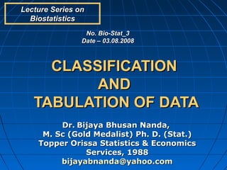
  • 1. Lecture Series on Biostatistics No. Bio-Stat_3 Date – 03.08.2008 CLASSIFICATION AND TABULATION OF DATA Dr. Bijaya Bhusan Nanda, M. Sc (Gold Medalist) Ph. D. (Stat.) Topper Orissa Statistics & Economics Services, 1988 bijayabnanda@yahoo.com
  • 2. LEARNING OBJECTIVES  The trainees will be able to do meaningful classification of large mass of data and interpret the same.  They will be able to construct frequency distribution table and interpret the same.  They will be able to describe different parts of tables and types of table
  • 3. CONTENT  Concept of Variable  Ordered array  What is data Classification ?  Objectives of Classification  Frequency distributions  Variables and attributes  Tabulation of data  Parts of a table  Type of tables
  • 4. Concept of Variable  Variable A characteristic which takes on different values in different persons, place or things. Example: Diastolic/Systolic blood pressure, heart rate, the heights of adult males, the weights of preschool children and the ages of patients seen in a dental clinic
  • 5. Quantitative Variable:- One that can be measured and expressed numerically. The measurements convey information regarding amount. Example: Diastolic/Systolic blood pressure, heart rate, the heights of adult males, the weights of preschool children and the ages of patients seen in a dental clinic  Qualitative Variable:- The characteristics that can’t be measured quantitatively but can be categorized. The measurement convey information regarding the attribute. The measurement in real sense can’t be achieved but persons, places or things belonging to different categories can be counted. Example: sex of a patient, colure and odour of stool and urine samples etc.
  • 6. Random Variable  Values obtained arise as a result of chance event/factor, so that can’t be exactly predicted in advance. Example: heights of a group of randomly selected adult.  Discrete Random Variable:- Characterized by gaps or interrupts in the values that it can assume. It assumes values with definite jumps. It can’t take all possible values within a range. It is observed through counting only Example: No. of daily admission to a general hospital, the no. of decayed, missing or filled teeth per child in an elementary school.
  • 7. Continuous Random Variable:- • It can take all possible values positive, negative, integral and fractional values within a specified relevant interval. • Doesn’t possess the gaps or interruptions within a specified relevant interval of values assumed by the variable. • Derived through measurement Example: height, weight and skull circumference Because of limitations of available measuring instruments, however observations on variables that are inherently continuous are recorded as if they are discrete.
  • 8. The ordered array  A first step in organizing data is preparation of an ordered array.  It is a listing of values of a data series from the smallest to the largest values.  It enables one to quickly determine the smallest and largest value in the data set and other facts about the arrayed data that might be needed in a hurried manner.  Look at the unordered and ordered data in the file DataExample.xls
  • 9. DATA CLASSIFICATION: The grouping of related facts/data into different classes according to certain common characteristic.  Basis of data Classification: • Broadly 4 broad basis 1. Geographical i.e. area wise • Total Population of Orissa by districts • No. of death due to malaria by districts. • Infant deaths in Orissa by districts
  • 10. 2. Chronological or Temporal • i.e. on the basis of time Table: 2 Death by lightening Year Number 1990 10 1991 5 1992 12 1993 6 1994 9 1995 3 1996 3 1997 5 1998 12 1999 12 2000 8 2001 7 2002 8 Total 100
  • 11. 3. Qualitative i.e. on the basis of some attributes Example: People by place of residence, sex and literacy Place of residence Rural Urban Male Female Male Female Literate Illiterate Literate Illiterate Literat Illiterate Literate Illiterate e
  • 12. 4. Quantitative: On the basis of quantitative class intervals For example students of a college may be classified according to weight as follows Table 3 :Weight of students of a college Wt. In (LBS) No. of students 90-100 50 100-110 200 110-120 260 120-130 360 130-140 90 140-150 40 Total 1000
  • 13. Classification of Age of 600 person in the Social Survey Class Relative Interval Frequency frequency 15 -24 56 09.3 25-34 153 25.5 35-44 149 24.8 45-54 75 12.5 55 - 64 61 10.2 65 - 74 70 11.7 75 - 84 28 4.7 85 - 94 8 1.3 Total 600 100.0
  • 14. In a survey of 35 families in a village, the number of children per family was recorded data were obtained. 1 0 2 3 4 5 6 7 2 3 4 0 2 5 8 4 5 9 6 3 2 7 6 5 3 3 7 8 9 7 9 4 5 4 3
  • 15. OBJECTIVES OF CLASSIFICATION  Helps in condensing the mass of data such that similarities and dissimilarities can be readily distinguished. No. of No of Cum. Fre. Cum. children families Less than Fre. (Frequency) Greater than 0-2 7 7 35 3-5 16 23 28 6 and 12 35 12 above Total 35
  • 16. Facilitate comparison No. of No of Cum. Fre. Cum. children families Less than Fre. (Frequency) Greater than 0-2 7 7 (20%) 35 (100) 3-5 16 23 28 (65.7%) (80%) 6 and 12 35 12 above (100%) (34%) Total 35
  • 17. Most significant features of the data can be pin pointed at a glance  Enables statistical treatment of the collected data  Averages can be computed  Variations can be revealed  Association can be studied  Model for prediction / forecasting can be built  Hypothesis can be formulated and tested etc.
  • 18. Principles of Classification: There is no hard and fast rules for deciding the class interval, however it depends upon:  Knowledge of the data  Lowest and highest value of the set of observations  Utility of the class intervals for meaningful comparison and interpretation r
  • 19. The classes should be collectively exhaustive and non-overlapping i.e. mutually exclusive.  The number of classes should not be too large other wise the purpose of class i.e. summarization of data will not be served.  The number of classes should not be too small either, for this also may obscure the true nature of the distribution.  The class should preferable of equal width. Other wise the class frequency would not be comparable, and the computation of statistical measures will be laborious.
  • 20. More specifically Struges formula can be used to decide the no. of class interval; • K=1+3.322(log 10n ) Where k = no. of classes, n=no. of observation  The width of the class interval may be determined by dividing the range by k w= R k where R= difference between the highest and the lowest observation. w = width of the class interval  When the nature of data make them appropriate class interval width of 5 units, 10 units and width that are multiple of 10 tend to make the summarization more comprehensible. r
  • 21. Classification will be called exclusive (Continuous), when the class intervals are so fixed that the upper limit of one class is the lower limit of the next class and the upper limit is not included in the class. An example Income (Rs.) No. of families 1000 – 1100 = (1000 but under 15 1100) 1100 – 1200 = (1100 but under 25 1200) 1200 – 1300 = (1200 but under 10 1300) Total 50
  • 22. Classification will be inclusive (discontinuous) when the upper and lower limit of one class is include in that class itself Income (Rs.) No. of persons 1000 – 1099 = (1000 but < 50 1099) 1100 – 1199 = (1100 but < 100 1199) 1200 – 1299 = (1200 but < 200 1299) Total 300
  • 23. Discontinuous class interval can be made continuous by applying the Correction factor. Lower limit of 2nd Class – Upper limit of the 1st Class CF = 2 The correction factor is subtracted from the lower limit and added to the upper limit to make the class interval continuous.
  • 24. Frequency distributions  Quantitative Variables: • Discrete variable • Continuous variable  Qualitative variable (attributes)  The manner in which the total number of observations are distributed over different classes is called a frequency distribution.
  • 25. Frequency distribution of an attribute Table 4 : Results of survey on Awarenesson HIV / AIDs State of Number of  In 1993, 1674 Knowledge people inhabitants of Aware 620 Calcutta, Bombay Unaware 1054 and Madras were Total 1674 surveyed. Each was asked, among, other questions, Table 5 : Proportion of people Aware of HIV / whether he/she AIDS knew about the HIV State of Relative / AIDS. The results Knowledge frequency is tabulated. Aware 0.370 Unaware 0.630 Total 1.000
  • 26. Frequency distribution of a discrete variable  Data grouped in to classes and the number of cases which fall in each class are recorded Example: In a survey of 35 families in a village, the number of children per family was recorded data were obtained. 1 0 2 3 4 5 6 7 2 3 4 0 2 5 8 4 5 9 6 3 2 7 6 5 3 3 7 8 9 7 9 4 5 4 3
  • 27. Steps for frequency distribution • Find the largest & smallest value; those are 9 and 0 respectively. • Form a table with 10 classes for the 10 values 0,1,2……9 • Look at the given values of the variable one by one and for each value put a tally mark in the table against the appropriate class. • To facilitate counting, the tally marks are arranged in the blocks of five every fifth stroke being drawn across the proceeding four. This is done below.
  • 28. Table 6: Frequency Table Cumulative Cumulative No. of Frequency Frequency Tallies Frequency children Less than More than type type 0  2 2 35 1  1 3 33 2  4 7 32 3  13 28 6  4  5 18 22 5  5 23 17 6  3 26 12 7  4 30 9 8  2 32 5 9  3 35 3
  • 29. TABULATION OF DATA  Compress the data into rows and columns and relation can be understood.  Tabulation simplifies complex data, facilitate comparison, gives identify to the data and reveals pattern
  • 30. Different parts of a table  Table number  Title of the table  Caption: Column Heading  Stub : Row heading  Body : Contains data  Head notes: Some thing that is not explained in the title, caption, stubs can be explained in the head notes on the top of the table below the title.  Foot notes: Source of data, some exception in the data can be given in the foot notes.
  • 31. Table can be classified into 3 ways Type of table Characteristic Feature 1. Simple table only one characteristic is shown 2. Complex table a. Two way table shows two characteristics and is formed when either the stub or the caption is divided in to two co- ordinate parts b. Higher order When three or more characteristic are table represented in the same table, such a table is called higher order table 3. General and published by Govt. such as in the special purpose table statistical Abstract of India, or census reports are general purpose table
  • 32. Complex table Average Number of OPD patients in a PHC in a tribal area in different age group according of sex OPD Patients Age in yrs Male Female Total Below 25 25 5 30 25-35 30 4 34 35-45 25 5 30 45-55 22 3 25 Above 55 15 1 16 Total 117 18 135
  • 33. Number of patients in OPDs of Public sector hospital by Religion, Age, Rank and Sex Religion Age(in yr.) Rank Supervisor Assistant Clerks Total F M T F M T F M T FMT Hindu Below 25 25- 35 35 – 45 45 – 55 55 & above Muslim Below 25 25- 35 35 – 45 45 – 55 55 & above Total
  • 34. Exercise Age of 169 subjects who participated in a study of Sparteine and Mephynytoin Oxidation is given. Calculate the frequency, cumulative frequency both less than and more than type, relative frequency and cumulative relative frequency. From these find out what is the proportion of patient aged 60 and more. (Data in the file DataExample.xls)
  • 35. Next Class: • Understanding data through presentations