Multiple Bifurcations of Sample Dynamical Systems

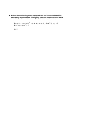
1.  A three-dimensional system, with quadratic and cubic nonlinearities,
affected by imperfections, undergoing a double-zero bifurcation. MSM.
..   2  
q 1   q 1  q1  b1 q 1  c1 q1 q2  b2 q1 q 1  b3 q1 2 q 1    0

q 2  kq2  c2 q1 2  0
k0

2. 2 4project_final_result.nb
Time scales and definitions
OffGeneral::spell1
 Notation`
Time scales
SymbolizeT0 ; SymbolizeT1 ; SymbolizeT2 ; SymbolizeT3 ; SymbolizeT4 ;
timeScales  T0 , T1 , T2 , T3 , T4 ;
dt1expr_ : Sum 2 Dexpr, timeScalesi  1, i, 0, maxOrder;
i
dt2expr_ : dt1dt1expr  Expand . i_;imaxOrder  0;
conjugateRule  A  A, A  A,   ,   , Complex0, n_  Complex0,  n;
displayRule  q_i_,j_ a__ __  RowTimes  MapIndexedD1
211 &, a, qi,j ,
A_i_ a__ __  RowTimes  MapIndexedD1
21 &, a, Ai , q_i_,j_ __  qi,j , A_i_ __  Ai ;

3. 4project_final_result.nb 3
Equations of motions
Equations of motion
EOM 
  b3 Subscriptq, 1t2 Subscriptq, 1 't  b2 Subscriptq, 1 't Subscriptq, 1t 
c1 Subscriptq, 2t Subscriptq, 1t  b1 Subscriptq, 1t2 
 Subscriptq, 1 't   Subscriptq, 1t  Subscriptq, 1 ''t  0,
c2 Subscriptq, 1t2  k Subscriptq, 2t  Subscriptq, 2 't  0; EOM  TableForm
   q1 t  b1 q1 t2  c1 q1 t q2 t   q1  t  b2 q1 t q1  t  b3 q1 t2 q1  t  q1  t  0
c2 q1 t2  k q2 t  q2  t  0
Ordering of the dampings
smorzrule     ,    ;
ombrule    3 
  3 
Definition of the expansion of qi
solRule  qi_  Sum qi,j1 1, 2, 3, 4, 5, j, 0, 5 &;
j
2
multiScales 
qi_ t  qi  timeScales, Derivativen_q_t  dtnq  timeScales, t  T0 ;
Max order of the procedure
maxOrder  4;

4. 4 4project_final_result.nb
Expansion and scaling of the equation
q1 T0 , T1 , T2 , T3 , T4 , T5  . solRule
q1,1 T0 , T1 , T2 , T3 , T4    q1,2 T0 , T1 , T2 , T3 , T4    q1,3 T0 , T1 , T2 , T3 , T4  
32 q1,4 T0 , T1 , T2 , T3 , T4   2 q1,5 T0 , T1 , T2 , T3 , T4   52 q1,6 T0 , T1 , T2 , T3 , T4 
q1 't . multiScales
2 q1 0,0,0,0,1 T0 , T1 , T2 , T3 , T4  
32 q1 0,0,0,1,0 T0 , T1 , T2 , T3 , T4    q1 0,0,1,0,0 T0 , T1 , T2 , T3 , T4  
 q1 0,1,0,0,0 T0 , T1 , T2 , T3 , T4   q1 1,0,0,0,0 T0 , T1 , T2 , T3 , T4 
Scaling of the variables
scaling  Subscriptq, 1t   Subscriptq, 1t,
Subscriptq, 2t   Subscriptq, 2t, Subscriptq, 1 't   Subscriptq, 1 't,
Subscriptq, 2 't   Subscriptq, 2 't, Subscriptq, 1 ''t 
 Subscriptq, 1 ''t, Subscriptq, 2 ''t   Subscriptq, 2 ''t
q1 t   q1 t, q2 t   q2 t, q1  t   q1  t,
q2  t   q2  t, q1  t   q1  t, q2  t   q2  t
Modification of the equations of motion : substitution of the rules.Representation.
EOMa 
EOM . scaling . multiScales . smorzrule . ombrule . solRule  TrigToExp  ExpandAll .
n_;n3  0; EOMa . displayRule
3   2  D0 q1,1  52  D0 q1,2  3  D0 q1,3   D2 q1,1  32 D2 q1,2  2 D2 q1,3  52 D2 q1,4  3 D2 q1,5 
0 0 0 0 0
52  D1 q1,1  3  D1 q1,2  2 32 D0 D1 q1,1  2 2 D0 D1 q1,2  2 52 D0 D1 q1,3  2 3 D0 D1 q1,4  2 D2 q1,1 
1
52 D2 q1,2  3 D2 q1,3  3  D2 q1,1  2 2 D0 D2 q1,1  2 52 D0 D2 q1,2  2 3 D0 D2 q1,3  2 52 D1 D2 q1,1 
1 1
2 3 D1 D2 q1,2  3 D2 q1,1  2 52 D0 D3 q1,1  2 3 D0 D3 q1,2  2 3 D1 D3 q1,1  2 3 D0 D4 q1,1  2  q1,1 
2
2 D0 q1,1 b2 q1,1  52 D0 q1,2 b2 q1,1  3 D0 q1,3 b2 q1,1  52 D1 q1,1 b2 q1,1  3 D1 q1,2 b2 q1,1 
3 D2 q1,1 b2 q1,1  2 b1 q2  3 D0 q1,1 b3 q2  52  q1,2  52 D0 q1,1 b2 q1,2  3 D0 q1,2 b2 q1,2 
1,1 1,1
3 D1 q1,1 b2 q1,2  2 52 b1 q1,1 q1,2  3 b1 q2  3  q1,3  3 D0 q1,1 b2 q1,3  2 3 b1 q1,1 q1,3 
1,2
2 c1 q1,1 q2,1  52 c1 q1,2 q2,1  3 c1 q1,3 q2,1  52 c1 q1,1 q2,2  3 c1 q1,2 q2,2  3 c1 q1,1 q2,3  0,
 D0 q2,1  32 D0 q2,2  2 D0 q2,3  52 D0 q2,4  3 D0 q2,5  32 D1 q2,1  2 D1 q2,2  52 D1 q2,3 
3 D1 q2,4  2 D2 q2,1  52 D2 q2,2  3 D2 q2,3  52 D3 q2,1  3 D3 q2,2  3 D4 q2,1  2 c2 q2 
1,1
2 52 c2 q1,1 q1,2  3 c2 q2  2 3 c2 q1,1 q1,3  k  q2,1  k 32 q2,2  k 2 q2,3  k 52 q2,4  k 3 q2,5  0
1,2

5. 4project_final_result.nb 5
EOMb  ExpandEOMa1, 1     0, ExpandEOMa2, 1     0; EOMb . displayRule
52   32  D0 q1,1  2  D0 q1,2  52  D0 q1,3   D2 q1,1   D2 q1,2  32 D2 q1,3  2 D2 q1,4 
0 0 0 0
52 D2 q1,5  2  D1 q1,1  52  D1 q1,2  2  D0 D1 q1,1  2 32 D0 D1 q1,2  2 2 D0 D1 q1,3 
0
2 52 D0 D1 q1,4  32 D2 q1,1  2 D2 q1,2  52 D2 q1,3  52  D2 q1,1  2 32 D0 D2 q1,1  2 2 D0 D2 q1,2 
1 1 1
2 52 D0 D2 q1,3  2 2 D1 D2 q1,1  2 52 D1 D2 q1,2  52 D2 q1,1  2 2 D0 D3 q1,1  2 52 D0 D3 q1,2 
2
2 52 D1 D3 q1,1  2 52 D0 D4 q1,1  32  q1,1  32 D0 q1,1 b2 q1,1  2 D0 q1,2 b2 q1,1 
52 D0 q1,3 b2 q1,1  2 D1 q1,1 b2 q1,1  52 D1 q1,2 b2 q1,1  52 D2 q1,1 b2 q1,1  32 b1 q2 
1,1
52 D0 q1,1 b3 q2  2  q1,2  2 D0 q1,1 b2 q1,2  52 D0 q1,2 b2 q1,2  52 D1 q1,1 b2 q1,2 
1,1
2 2 b1 q1,1 q1,2  52 b1 q2  52  q1,3  52 D0 q1,1 b2 q1,3  2 52 b1 q1,1 q1,3  32 c1 q1,1 q2,1 
1,2
2 c1 q1,2 q2,1  52 c1 q1,3 q2,1  2 c1 q1,1 q2,2  52 c1 q1,2 q2,2  52 c1 q1,1 q2,3  0,
 D0 q2,1   D0 q2,2  32 D0 q2,3  2 D0 q2,4  52 D0 q2,5   D1 q2,1  32 D1 q2,2  2 D1 q2,3  52 D1 q2,4 
32 D2 q2,1  2 D2 q2,2  52 D2 q2,3  2 D3 q2,1  52 D3 q2,2  52 D4 q2,1  32 c2 q2  2 2 c2 q1,1 q1,2 
1,1
52 c2 q2  2 52 c2 q1,1 q1,3  k
1,2  q2,1  k  q2,2  k 32 q2,3  k 2 q2,4  k 52 q2,5  0
Separation of the coefficients of the powers of 
eqEps  RestThreadCoefficientListSubtract  ,  2   0 &  EOMb  Transpose;
1
Definition of the equations at orders of  and representation
eqOrderi_ : 1 &  eqEps1 . q_k_,1  qk,i  
1 &  eqEps1 . q_k_,1  qk,i   1 &  eqEpsi  Thread

6. 6 4project_final_result.nb
Pertubation equations
.
.
eqOrder1 displayRule
.
eqOrder2 displayRule
.
eqOrder3 displayRule
.
eqOrder4 displayRule
eqOrder5 displayRule
D2 q1,1  0, D0 q2,1  k q2,1  0
0
D2 q1,2   2 D0 D1 q1,1 , D0 q2,2  k q2,2   D1 q2,1 
0
D2 q1,3   D0 q1,1  2 D0 D1 q1,2  D2 q1,1  2 D0 D2 q1,1   q1,1  D0 q1,1 b2 q1,1  b1 q2  c1 q1,1 q2,1 ,
D0 q2,3  k q2,3   D1 q2,2  D2 q2,1  c2 q2 
0 1 1,1
1,1
D2 q1,4   D0 q1,2   D1 q1,1  2 D0 D1 q1,3  D2 q1,2  2 D0 D2 q1,2  2 D1 D2 q1,1  2 D0 D3 q1,1 
0 1
D0 q2,4  k q2,4   D1 q2,3  D2 q2,2  D3 q2,1  2 c2 q1,1 q1,2 
D0 q1,2 b2 q1,1  D1 q1,1 b2 q1,1   q1,2  D0 q1,1 b2 q1,2  2 b1 q1,1 q1,2  c1 q1,2 q2,1  c1 q1,1 q2,2 ,
D2 q1,5 
0
    D0 q1,3   D1 q1,2  2 D0 D1 q1,4  D2 q1,3   D2 q1,1  2 D0 D2 q1,3  2 D1 D2 q1,2  D2 q1,1  2 D0 D3 q1,2 
1 2
2 D1 D3 q1,1  2 D0 D4 q1,1  D0 q1,3 b2 q1,1  D1 q1,2 b2 q1,1  D2 q1,1 b2 q1,1  D0 q1,1 b3 q2  D0 q1,2 b2 q1,2 
1,1
D0 q2,5  k q2,5   D1 q2,4  D2 q2,3  D3 q2,2  D4 q2,1  c2 q2  2 c2 q1,1 q1,3 
D1 q1,1 b2 q1,2  b1 q2   q1,3  D0 q1,1 b2 q1,3  2 b1 q1,1 q1,3  c1 q1,3 q2,1  c1 q1,2 q2,2  c1 q1,1 q2,3 ,
1,2
1,2

7. 4project_final_result.nb 7
First  Order Problem
Equations  0)
linearSys  1 &  eqOrder1;
linearSys . displayRule  TableForm
D2 q1,1
0
D0 q2,1  k q2,1
Formal solution of the First  Order Problem generating solution
sol1  q1,1  FunctionT0 , T1 , T2 , T3 , T4 , A1 T1 , T2 , T3 , T4  ,
q2,1  FunctionT0 , T1 , T2 , T3 , T4 , 0
q1,1  FunctionT0 , T1 , T2 , T3 , T4 , A1 T1 , T2 , T3 , T4 , q2,1  FunctionT0 , T1 , T2 , T3 , T4 , 0

8. 8 4project_final_result.nb
Second  Order Problem
Substitution of the solution on the Second  Order Problem and representation
eqOrder2 . displayRule
D2 q1,2   2 D0 D1 q1,1 , D0 q2,2  k q2,2   D1 q2,1 
0
order2Eq  eqOrder2 . sol1  ExpandAll;
order2Eq . displayRule
D2 q1,2  0, D0 q2,2  k q2,2  0
0
we eliminate secular terms then we obtain
sol2  q1,2  FunctionT0 , T1 , T2 , T3 , T4 , 0 , q2,2  FunctionT0 , T1 , T2 , T3 , T4 , 0
q1,2  FunctionT0 , T1 , T2 , T3 , T4 , 0, q2,2  FunctionT0 , T1 , T2 , T3 , T4 , 0

9. 4project_final_result.nb 9
Third  Order Problem
Substitution in the Third  Order Equations
order3Eq  eqOrder3 . sol1 . sol2  ExpandAll;
order3Eq . displayRule
D2 q1,3   D2 A1   A1  A2 b1 , D0 q2,3  k q2,3   A2 c2 
0 1 1 1
ST31  order3Eq, 2 &  1;
ST31 . displayRule
 D2 A1   A1  A2 b1 
1 1
SCond3  ST31  0;
SCond3 . displayRule
 D2 A1   A1  A2 b1   0
1 1
SCond3
 A1 T1 , T2 , T3 , T4   b1 A1 T1 , T2 , T3 , T4 2  A1 2,0,0,0 T1 , T2 , T3 , T4   0
SCond3Rule1 
SolveSCond3, A1 2,0,0,0 T1 , T2 , T3 , T4 1  ExpandAll  Simplify  Expand;
SCond3Rule1 . displayRule
D2 A1   A1  A2 b1 
1 1
sol3  q1,3  FunctionT0 , T1 , T2 , T3 , T4 , 0 ,
q2,3  FunctionT0 , T1 , T2 , T3 , T4 ,  A1 T1 , T2 , T3 , T4 2 c2  k
q1,3  FunctionT0 , T1 , T2 , T3 , T4 , 0,
A1 T1 , T2 , T3 , T4 2 c2
q2,3  FunctionT0 , T1 , T2 , T3 , T4 ,  
k

10. 10 4project_final_result.nb
Fourth  Order Problem
Substitution in the Fourth  Order Equations
order4Eq  eqOrder4 . sol1 . sol2 . sol3  ExpandAll;
order4Eq . displayRule
D2 q1,4   D1 A1  2 D1 D2 A1  D1 A1 A1 b2 , D0 q2,4  k q2,4  
2 D1 A1 A1 c2
0
k
ST41  order4Eq, 2 &  1;
ST41 . displayRule
 D1 A1  2 D1 D2 A1  D1 A1 A1 b2 
SCond4  ST41  0;
SCond4 . displayRule
 D1 A1  2 D1 D2 A1  D1 A1 A1 b2   0
SCond4
 A1 1,0,0,0 T1 , T2 , T3 , T4  
b2 A1 T1 , T2 , T3 , T4  A1 1,0,0,0 T1 , T2 , T3 , T4   2 A1 1,1,0,0 T1 , T2 , T3 , T4   0
SCond4Rule1 
SolveSCond4, A1 1,1,0,0 T1 , T2 , T3 , T4 1  ExpandAll  Simplify  Expand;
SCond4Rule1 . displayRule
D1 D2 A1  D1 A1 A1 b2 
 D1 A1 1

2 2
SCond3Rule1 . displayRule
D2 A1   A1  A2 b1 
1 1
SCond3Rule1
A1 2,0,0,0 T1 , T2 , T3 , T4    A1 T1 , T2 , T3 , T4   b1 A1 T1 , T2 , T3 , T4 2 
SCond4Rule1
A1 1,1,0,0 T1 , T2 , T3 , T4  
 A1 1,0,0,0 T1 , T2 , T3 , T4   b2 A1 T1 , T2 , T3 , T4  A1 1,0,0,0 T1 , T2 , T3 , T4 
1 1
2 2

11. 4project_final_result.nb 11
2 A1 1,1,0,0 T1 , T2 , T3 , T4   A1 2,0,0,0 T1 , T2 , T3 , T4  . SCond3Rule1 . SCond4Rule1
 A1 T1 , T2 , T3 , T4   b1 A1 T1 , T2 , T3 , T4 2 
 A1 1,0,0,0 T1 , T2 , T3 , T4   b2 A1 T1 , T2 , T3 , T4  A1 1,0,0,0 T1 , T2 , T3 , T4 
1 1
2
2 2
TimeRule1  A1 T1 , T2 , T3 , T4   A1 t, A1 1,0,0,0 T1 , T2 , T3 , T4   A1 't 
A1 T1 , T2 , T3 , T4   A1 t, A1 1,0,0,0 T1 , T2 , T3 , T4   A1  t
2 A1 1,1,0,0 T1 , T2 , T3 , T4   A1 2,0,0,0 T1 , T2 , T3 , T4  . SCond3Rule1 . SCond4Rule1 .
TimeRule1  A1 ''t
 A1 t  b1 A1 t2  2  A1  t  b2 A1 t A1  t  A1  t
1 1
2 2
sol4  q1,4  FunctionT0 , T1 , T2 , T3 , T4 , 0 ,
2 D1 A1 T1 , T2 , T3 , T4  A1 T1 , T2 , T3 , T4  c2
q2,4  FunctionT0 , T1 , T2 , T3 , T4 , 
k
q1,4  FunctionT0 , T1 , T2 , T3 , T4 , 0,
2 D1 A1 T1 , T2 , T3 , T4  A1 T1 , T2 , T3 , T4  c2
q2,4  FunctionT0 , T1 , T2 , T3 , T4 , 
k

12. 12 4project_final_result.nb
Fifth  Order Problem
order5Eq  eqOrder5 . sol1 . sol2 . sol3 . sol4  ExpandAll;
order5Eq . displayRule
D2 q1,5      D2 A1  D2 A1  2 D1 D3 A1  D2 A1 A1 b2 
A3 c1 c2
1
0 2 ,
2 D1 A1 c2 D1 A1 T1 , T2 , T3 , T4  2 A1 c2 D1 A1 1,0,0,0 T1 , T2 , T3 , T4 
k

2 D2 A1 A1 c2
D0 q2,5  k q2,5   
k k k
ST51  order5Eq, 2 &  1;
ST51 . displayRule
    D2 A1  D2 A1  2 D1 D3 A1  D2 A1 A1 b2  
A3 c1 c2
1
2
k
SCond5  ST51  0;
SCond5 . displayRule
    D2 A1  D2 A1  2 D1 D3 A1  D2 A1 A1 b2  0
A3 c1 c2
1
2
k
SCond5
c1 c2 A1 T1 , T2 , T3 , T4 3
   
 A1 0,1,0,0 T1 , T2 , T3 , T4   b2 A1 T1 , T2 , T3 , T4  A1 0,1,0,0 T1 , T2 , T3 , T4  
k
A1 0,2,0,0 T1 , T2 , T3 , T4   2 A1 1,0,1,0 T1 , T2 , T3 , T4   0
SCond5Rule1 
SolveSCond5, A1 0,2,0,0 T1 , T2 , T3 , T4  1  ExpandAll  Simplify  Expand;
SCond5Rule1 . displayRule
D2 A1      D2 A1  2 D1 D3 A1  D2 A1 A1 b2  
A3 c1 c2
1
2
k
SCond5Rule1
c1 c2 A1 T1 , T2 , T3 , T4 3
A1 0,2,0,0 T1 , T2 , T3 , T4        A1 0,1,0,0 T1 , T2 , T3 , T4  
b2 A1 T1 , T2 , T3 , T4  A1 0,1,0,0 T1 , T2 , T3 , T4   2 A1 1,0,1,0 T1 , T2 , T3 , T4 
k
A1 0,2,0,0 T1 , T2 , T3 , T4   2 A1 1,0,1,0 T1 , T2 , T3 , T4  . SCond5Rule1 . TimeRule1
c1 c2 A1 t3
    A1 0,1,0,0 T1 , T2 , T3 , T4   b2 A1 t A1 0,1,0,0 T1 , T2 , T3 , T4 
k

13. 4project_final_result.nb 13
sol5  q1,5  FunctionT0 , T1 , T2 , T3 , T4 , 0 , q2,5  FunctionT0 , T1 , T2 , T3 , T4 ,
2 D1 A1 c2 D1 A1 T1 , T2 , T3 , T4  2 A1 c2 D1 A1 1,0,0,0 T1 , T2 , T3 , T4 

2 D2 A1 A1 c2
 
k2 k2 k2
q1,5  FunctionT0 , T1 , T2 , T3 , T4 , 0, q2,5  FunctionT0 , T1 , T2 , T3 , T4 ,
2 D1 A1 c2 D1 A1 T1 , T2 , T3 , T4  2 A1 c2 D1 A1 1,0,0,0 T1 , T2 , T3 , T4 

2 D2 A1 A1 c2
 
k2 k2 k2

14. 14 4project_final_result.nb
Bifurcation equations and fixed points
TimeRule2  A1 0,1,0,0 T1 , T2 , T3 , T4   0
A1 0,1,0,0 T1 , T2 , T3 , T4   0
RBFCE  A1 0,2,0,0 T1 , T2 , T3 , T4   2 A1 1,0,1,0 T1 , T2 , T3 , T4  
2 A1 1,1,0,0 T1 , T2 , T3 , T4   A1 2,0,0,0 T1 , T2 , T3 , T4  . SCond3Rule1 .
SCond4Rule1 . SCond5Rule1 . TimeRule1 . TimeRule2  A1 ''t
c1 c2 A1 t3
    A1 t  b1 A1 t2   A1  t  b2 A1 t A1  t  A1  t
1 1
2
k 2 2
IF we neglected the contribution of the passive variable the bifurcation equation becomes
MBFCE  A1 0,2,0,0 T1 , T2 , T3 , T4   2 A1 1,0,1,0 T1 , T2 , T3 , T4   2 A1 1,1,0,0 T1 , T2 , T3 , T4  
c1 c2 A1 T1 , T2 , T3 , T4 3
A1 2,0,0,0 T1 , T2 , T3 , T4   . SCond3Rule1 .
k
SCond4Rule1 . SCond5Rule1 . TimeRule1 . TimeRule2  A1 ''t
    A1 t  b1 A1 t2  2  A1  t  b2 A1 t A1  t  A1  t
1 1
2 2

15. 4project_final_result.nb 15
Fixed points both for the
perfect and imperfect system
Perfect system
perfectsyst    0, A1  t  0, A1  t  0 
  0, A1  t  0, A1  t  0
fix1  MBFCE . perfectsyst
 A1 t  b1 A1 t2
fixpoint1  fix1  0;
fixpoint1 . displayRule
 A1  A2 b1  0
1
fixpoint1
 A1 t  b1 A1 t2  0
Imperfect system
imperfectsyst  A1  t  0, A1  t  0 
A1  t  0, A1  t  0
fix2  MBFCE . imperfectsyst
    A1 t  b1 A1 t2
fixpoint2  fix2  0;
fixpoint2 . displayRule
    A1  A2 b1  0
1
fixpoint2
    A1 t  b1 A1 t2  0
scalingRule2   A1 2,0,0,0 T1 , T2 , T3 , T4   A1  t 
A1 2,0,0,0 T1 , T2 , T3 , T4   A1  t

16. 16 4project_final_result.nb
Reconstitution of the equation of the motion
Stepx1  A1 T1 , T2 , T3 , T4 
A1 T1 , T2 , T3 , T4 
Stepy1 
2 D2 A1 T1 , T2 , T3 , T4  A1 T1 , T2 , T3 , T4  c2 2 D1 A1 T1 , T2 , T3 , T4  c2 D1 A1 T1 , T2 , T3 , T4 
 
k2 k2
2 A1 T1 , T2 , T3 , T4  c2 D1 A1 1,0,0,0 T1 , T2 , T3 , T4 

k2
2 D1 A1 T1 , T2 , T3 , T4  A1 T1 , T2 , T3 , T4  c2 A1 T1 , T2 , T3 , T4 2 c2
 
k k
2 c2 D1 A1 T1 , T2 , T3 , T4 2 2 c2 D1 A1 T1 , T2 , T3 , T4  A1 T1 , T2 , T3 , T4 
  
2 c2 D2 A1 T1 , T2 , T3 , T4  A1 T1 , T2 , T3 , T4  c2 A1 T1 , T2 , T3 , T4 2
k2 k
 
2 c2 A1 T1 , T2 , T3 , T4  D1 A1 1,0,0,0 T1 , T2 , T3 , T4 
k2 k
k2
ScalingRule1  A1 T1 , T2 , T3 , T4   A1 t
A1 T1 , T2 , T3 , T4   A1 t
x t  A1 T1 , T2 , T3 , T4  . ScalingRule1
Set::write : Tag Times in t x is Protected. 
A1 t
scalingRule2 
 D1 A1 1,0,0,0 T1 , T2 , T3 , T4   A1  t , D2 A1 T1 , T2 , T3 , T4   0 , D1 A1 T1 , T2 , T3 , T4   A1  t
D1 A1 1,0,0,0 T1 , T2 , T3 , T4   A1  t, D2 A1 T1 , T2 , T3 , T4   0, D1 A1 T1 , T2 , T3 , T4   A1  t

17. 4project_final_result.nb 17
2 c2 D1 A1 T1 , T2 , T3 , T4 2 2 c2 D1 A1 T1 , T2 , T3 , T4  A1 T1 , T2 , T3 , T4 
y t    
k2 k
2 c2 D2 A1 T1 , T2 , T3 , T4  A1 T1 , T2 , T3 , T4  c2 A1 T1 , T2 , T3 , T4 2
 
k2 k
2 c2 A1 T1 , T2 , T3 , T4  D1 A1 1,0,0,0 T1 , T2 , T3 , T4 
. scalingRule2 . ScalingRule1
k2
Set::write : Tag Times in t y is Protected. 
c2 A1 t2 2 c2 A1 t A1  t 2 c2 A1  t2 2 c2 A1 t A1  t
   
k k k2 k2

18. 18 4project_final_result.nb
Numerical integrations
Numerical values for the perfect system
c1  1, k  2, b3 
1
, b1  1, b2  1, c2  1,   0.01,    0.09,   0
2
1, 2,
1
, 1, 1, 1, 0.01,  0.09, 0
2
Time of integration
ti  500;
Numerical Intergations of the reconstitute
solution and study of the motion around the equilibrium points
solramep1  NDSolveMBFCE  0, A1 0  0.01, A1  0  0.01 ,
A1 t, A1  t, A1  t, t, 0, ti
NDSolve::ndsz : At t  74.65045623139203`, step size is effectively zero; singularity or stiff system suspected. 
A1 t  InterpolatingFunction0., 74.6505, t,
A1  t  InterpolatingFunction0., 74.6505, t,
A1  t  InterpolatingFunction0., 74.6505, t

19. 4project_final_result.nb 19
GraphicsArrayPlotA1 t . solramep1, t, 0, ti, PlotStyle  Thick,
PlotRange  Automatic,  3.8, 3.8, Frame  True, FrameLabel  "t", "xt",
PlotA1  t . solramep1, t, 0, ti, PlotStyle  Thick,
PlotRange  Automatic,  3.6, 3.4, Frame  True, FrameLabel  "t", "x't"
ParametricPlotA1 t . solramep1, A1  t . solramep1, t, 0, 25, PlotStyle  Thick,
PlotRange  Automatic,  0.6, 0.4, Frame  True, FrameLabel  "xt", "x't" 
3 3
2 2
1 1
xt
x't
0 0
1 1
2 2
3 3
0 100 200 300 400 500 0 100 200 300 400 500
t t
0.4
0.2
0.0
x't
0.2
0.4
0.6
0.0 0.2 0.4 0.6 0.8 1.0
xt
Graphics of the reconstituted solution

20. 20 4project_final_result.nb
solramep1  NDSolveRBFCE  0, A1 0  0.01, A1  0  0.01 ,
A1 t, A1  t, A1  t, t, 0, ti
GraphicsArrayPlotA1 t . solramep1, t, 0, ti, PlotStyle  Thick,
PlotRange  Automatic,  3.8, 3.8, Frame  True, FrameLabel  "t", "xt",
c2 A1 t2 2 c2 A1 t A1  t 2 c2 A1  t2 2 c2 A1 t A1  t
Plot     . solramep1,
k k k2 k2
t, 0, ti, PlotStyle  Thick, PlotRange  Automatic,  2.6, 2.4,
Frame  True, FrameLabel  "t", "yt"
NDSolve::ndsz : At t  73.98791597135596`, step size is effectively zero; singularity or stiff system suspected. 
A1 t  InterpolatingFunction0., 73.9879, t,
A1  t  InterpolatingFunction0., 73.9879, t,
A1  t  InterpolatingFunction0., 73.9879, t
3 2
2 1
1
xt
yt
0 0
1 1
2
3 2
0 100 200 300 400 500 0 100 200 300 400 500
t t
Numerical Intergations of the original equations
solorig1  NDSolveJoinEOM, q1 0  0.01, q2 0  0.01, q1 '0  0.01,
q1 t, q2 t, t, 0, ti, MaxSteps  1 000 000
NDSolve::nderr : Error test failure at t  95.2991109549007`; unable to continue. 
q1 t  InterpolatingFunction0., 95.2991, t,
q2 t  InterpolatingFunction0., 95.2991, t
GraphicsArrayPlotq1 t . solorig1, t, 0, ti, PlotStyle  Thick,
PlotRange  Automatic,  0.8, 0.8, Frame  True, FrameLabel  "t", "q1 t",
Plotq2 t . solorig1, t, 0, ti, PlotStyle  Thick,
PlotRange  Automatic,  0.6, 0.4, Frame  True, FrameLabel  "t", "q2 t"
0.4
0.5
0.2
q1 t
0.0
q2 t
0.0
0.2
0.5 0.4
0.6
0 100 200 300 400 500 0 100 200 300 400 500
t t
Numerical value for the imperfect system

21. 4project_final_result.nb 21
c1  1, k  2, b3 
1
, b1  1, b2  1, c2  1,   0.01,    0.01,   0.01  0.001
2
1, 2,
1
, 1, 1, 1, 0.01,  0.01, 0.00001
2
Numerical Intergations of the reconstitute
solution and study of the motion around the equilibrium points
solramep1  NDSolveMBFCE  0, A1 0  0.01, A1  0  0.01 ,
A1 t, A1  t, A1  t, t, 0, ti
NDSolve::ndsz : At t  26.093351632129746`, step size is effectively zero; singularity or stiff system suspected. 
A1 t  InterpolatingFunction0., 26.0934, t,
A1  t  InterpolatingFunction0., 26.0934, t,
A1  t  InterpolatingFunction0., 26.0934, t

22. 22 4project_final_result.nb
GraphicsArrayPlotA1 t . solramep1, t, 0, ti, PlotStyle  Thick,
PlotRange  Automatic,  3.8, 3.8, Frame  True, FrameLabel  "t", "xt",
PlotA1  t . solramep1, t, 0, ti, PlotStyle  Thick,
PlotRange  Automatic,  3.6, 3.4, Frame  True, FrameLabel  "t", "x't"
ParametricPlotA1 t . solramep1, A1  t . solramep1, t, 0, 25, PlotStyle  Thick,
PlotRange  Automatic,  0.6, 0.4, Frame  True, FrameLabel  "xt", "x't" 
3 3
2 2
1 1
xt
x't
0 0
1 1
2 2
3 3
0 100 200 300 400 500 0 100 200 300 400 500
t t
0.4
0.2
0.0
x't
0.2
0.4
0.6
0.0 0.2 0.4 0.6 0.8 1.0
xt
Graphics of the reconstituted solution
solramep1  NDSolveRBFCE  0, A1 0  0.01, A1  0  0.01 ,
A1 t, A1  t, A1  t, t, 0, ti
NDSolve::ndsz : At t  25.75990904121472`, step size is effectively zero; singularity or stiff system suspected. 
A1 t  InterpolatingFunction0., 25.7599, t,
A1  t  InterpolatingFunction0., 25.7599, t,
A1  t  InterpolatingFunction0., 25.7599, t

23. 4project_final_result.nb 23
GraphicsArrayPlotA1 t . solramep1, t, 0, ti, PlotStyle  Thick,
PlotRange  Automatic,  3.8, 3.8, Frame  True, FrameLabel  "t", "xt",
c2 A1 t2 2 c2 A1 t A1  t 2 c2 A1  t2 2 c2 A1 t A1  t
Plot     . solramep1,
k k k2 k2
t, 0, ti, PlotStyle  Thick, PlotRange  Automatic,  2.6, 2.4,
Frame  True, FrameLabel  "t", "yt"
3 2
2 1
1
xt
yt
0 0
1 1
2
3 2
0 100 200 300 400 500 0 100 200 300 400 500
t t
Numerical Intergations of the original equations
solorig1  NDSolveJoinEOM, q1 0  0.01, q2 0  0.01, q1 '0  0.01,
q1 t, q2 t, t, 0, ti, MaxSteps  1 000 000
NDSolve::nderr : Error test failure at t  43.327453744383035`; unable to continue. 
q1 t  InterpolatingFunction0., 43.3275, t,
q2 t  InterpolatingFunction0., 43.3275, t
GraphicsArrayPlotq1 t . solorig1, t, 0, ti, PlotStyle  Thick,
PlotRange  Automatic,  0.8, 0.8, Frame  True, FrameLabel  "t", "q1 t",
Plotq2 t . solorig1, t, 0, ti, PlotStyle  Thick,
PlotRange  Automatic,  0.6, 0.4, Frame  True, FrameLabel  "t", "q2 t"
0.4
0.5
0.2
q1 t
0.0
q2 t
0.0
0.2
0.5 0.4
0.6
0 100 200 300 400 500 0 100 200 300 400 500
t t
Proof that the system has an infinite value in finite time
c1  1, k  2, b3  4, b1  1, b2  1, c2  1,   0.01,   0.095,   0.01  0.001
1, 2, 4, 1, 1, 1, 0.01, 0.095, 0.00001

24. 24 4project_final_result.nb
solorig1  NDSolveJoinEOM, q1 0  0.01, q2 0  0.01, q1 '0  0.01,
q1 t, q2 t, t, 0, ti, MaxSteps  1 000 000
q1 t  InterpolatingFunction0., 500., t,
q2 t  InterpolatingFunction0., 500., t
GraphicsArrayPlotq1 t . solorig1, t, 0, ti, PlotStyle  Thick,
PlotRange  Automatic,  0.8, 0.8, Frame  True, FrameLabel  "t", "q1 t",
Plotq2 t . solorig1, t, 0, ti, PlotStyle  Thick,
PlotRange  Automatic,  0.6, 0.4, Frame  True, FrameLabel  "t", "q2 t"
0.4
0.5
0.2
q1 t
0.0
q2 t
0.0
0.2
0.5 0.4
0.6
0 100 200 300 400 500 0 100 200 300 400 500
t t