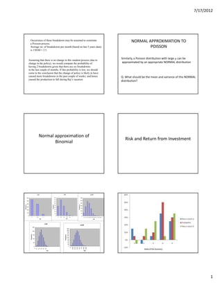
1. 7/17/2012
Occurrence of these breakdown may be assumed to constitute
a Poisson process.
NORMAL APPROXIMATION TO
Average no. of breakdowns per month (based on last 5 years data) POISSON
is 150/60 = 2.5.
Similarly, a Poisson distribution with large µ can be
Assuming that there is no change in this random process (due to
change in the policy), we would compute the probability of approximated by an appropriate NORMAL distribution
having 2 breakdowns given that there are six breakdowns
in the last couple of months. If this probability is low, we should
come to the conclusion that the change of policy is likely to have
caused more breakdowns in the past couple of weeks; and hence Q. What should be the mean and variance of this NORMAL
caused the production to fall during Raj’s vacation.
distribution?
Normal approximation of
Risk and Return from Investment
Binomial
n=2 n=5 n=10
600 450 350
400
500 300
350
250
400 300
Frequency
Frequency
Frequency
250 200
300
200
150
200 150
100
100
100
50 50
0 0 0
0 0.5 1 0 0.2 0.4 0.6 0.8 1 0 0.1 0.2 0.3 0.4 0.5 0.6 0.7 0.8 0.9 1
Bin Bin
Bin
n=20
n=25
250
200
180
200
160
140
Frequency
Frequency
150
120
100
100 80
60
50 40
20
0 0
0
0.08
0.16
0.24
0.32
0.4
0.48
0.56
0
1
2
3
4
5
0.
0.
0.
0.
0.
Bin Bin 25
1

2. 7/17/2012
Mean & Standard deviation of RETURN Covariance and Correlation between
(Stock X) return from Stocks X and Y
State of the X = Return Y= Return (x- mu_X)
economy p = Prob. stock X stock Y *(y-mu_Y) x*y
State of the p= X = Return from 1 0.05 15 -5 231 -75
economy Probability stock X (in %) (x -mu_X)^2 x^2 2 0.05 -5 15 31 -75
1 0.05 15 121 225 3 0.1 5 25 -189 125
4 0.5 35 5 -99 175
2 0.05 -5 961 25 5 0.3 25 35 -19 875
3 0.1 5 441 25
4 0.5 35 81 1225 mean 26 16 -61 355
5 0.3 25 1 625 variance 139 199
std dev 11.79 14.11 check
mean 26 139 815 covariance -61 355-26*16= -61
correlation -0.367
variance 139 815-26^2= 139
std dev 11.79
Expected Value / Standard Covariance and Correlation between
deviation of return from Stock returns from Stock A and Stock B
R B : retu rn fro m S to ck B is an o th er ran d o m variab le
RA : return from Stock A is a random variable
E x p ected valu e o f retu rn fro m S to ck B :
Expected value of return from Stock A: E (RB ) = ∑b i × p i = µ B , w h ere
i
E ( RA ) = ∑ ai × pi = µ A , where b i = retu rn fro m S to ck B w h en sta te o f th e eco n o m y is i
i
V arian ce o f retu rn fro m S to c k A :
pi = P(state of the economy is i) σ 2 = E (RB − µ B )2 =
B ∑ (b i − µ B ) 2 × pi = ∑ (b ) i
2
× pi − µ 2
B
i i
ai = return from Stock A when state of the economy is i C o varian ce b etw een retu rn s fro m S to ck A an d S to ck B :
Variance of return from Stock A: σ A B = E [ ( R A − µ A )( R B − µ B ) ] = ∑ (a i − µ A ) × ( bi − µ B ) × p i
i
σ 2 = E ( RA − µ A ) 2 = ∑ (ai − µ A ) 2 × pi = E [R A RB ] − µ Aµ B = ∑a i × bi × p i − µ A × µ B
A i
i
C o rrela tio n b etw een retu rn s fro m S to ck A an d S to ck B :
= E ( RA ) 2 − µ 2 = ∑ (ai ) 2 × pi − µ 2
A A ρ AB =
σ AB
i σA × σB
Mean and Standard deviation of Average Return and Std. Dev of return
RETURN from stock Y weight for
from a Portfolio
stock 0.8 0.2
P= portfolio (P-mu_P)^2
State of the p= Y= Return from
State of the X= Return Y= Return
return
economy p = Prob. stock X stock Y
economy Probability stock Y (in %) (y -mu_Y)^2 y^2
1 0.05 15 -5 11 169
1 0.05 -5 441 25
-1 625
2 0.05 -5 15
2 0.05 15 1 225 3 0.1 5 25 9 225
3 0.1 25 81 625 4 0.5 35 5 29 25
4 0.5 5 121 25 5 0.3 25 35 27 9
5 0.3 35 361 1225
mean 26 16 24 77.4
mean 16 199 455
variance 139 199 77.4
std dev 11.79 14.11 8.80
variance 199 455-16^2= 199
covariance -61 0.8*26+0.2*16
std dev 14.11
correlation -0.367 0.8^2 * 139 + 0.2^2 * 199+ 2*0.8*0.2 *(-61)
2

3. 7/17/2012
Risk and Return from Portfolio:
Diversification of Portfolio
Portfolio: Out of 1 unit, put w unit in A and (1- w) in B
Return from portfolio: P = w × RA + (1- w) × RB
Expected value of return from portfolio:
E ( P) = w × µ A + (1- w) × µ B
Variance of return from portfolio
σ 2 = w2 × σ A + (1 − w) 2 × σB + 2w(1 − w)σ AB
P
2 2
If the two returns are negatively correlated (negative covariance)
The portfolio may have reduced risk (standard deviation)
Portfolio Diversification and Asset
allocation
• The benefit of ‘diversification’
• The above formulae can be elegantly
formulated using matrix
• Computation using Excel
– Portfolio Diversification
– Data file
• Optimization technique
3