Top profile Call Girls In Hubli [ 7014168258 ] Call Me For Genuine Models We ...
Permanent Magnet Synchronous
1. Abstract
Julius Luukko
Direct torque control of permanent magnet synchronous machines – analysis and
implementation
Lappeenranta 2000
172 p.
Acta Universitatis Lappeenrantaensis 97
Diss. Lappeenranta University of Technology
ISBN 951-764-438-8, ISSN 1456-4491
The direct torque control (DTC) has become an accepted vector control method beside
the current vector control. The DTC was first applied to asynchronous machines, and
has later been applied also to synchronous machines. This thesis analyses the applica-
tion of the DTC to permanent magnet synchronous machines (PMSM).
In order to take the full advantage of the DTC, the PMSM has to be properly dimen-
sioned. Therefore the effect of the motor parameters is analysed taking the control prin-
ciple into account. Based on the analysis, a parameter selection procedure is presented.
The analysis and the selection procedure utilize nonlinear optimization methods.
The key element of a direct torque controlled drive is the estimation of the stator flux
linkage. Different estimation methods – a combination of current and voltage models
and improved integration methods – are analysed. The effect of an incorrect measured
rotor angle in the current model is analysed and an error detection and compensation
method is presented. The dynamic performance of an earlier presented sensorless flux
estimation method is made better by improving the dynamic performance of the low-
pass filter used and by adapting the correction of the flux linkage to torque changes.
A method for the estimation of the initial angle of the rotor is presented. The method
is based on measuring the inductance of the machine in several directions and fitting the
measurements into a model. The model is nonlinear with respect to the rotor angle and
therefore a nonlinear least squares optimization method is needed in the procedure.
A commonly used current vector control scheme is the minimum current control. In
the DTC the stator flux linkage reference is usually kept constant. Achieving the min-
imum current requires the control of the reference. An on-line method to perform the
minimization of the current by controlling the stator flux linkage reference is presented.
Also, the control of the reference above the base speed is considered.
A new estimation flux linkage is introduced for the estimation of the parameters of
the machine model. In order to utilize the flux linkage estimates in off-line parameter
estimation, the integration methods are improved. An adaptive correction is used in
the same way as in the estimation of the controller stator flux linkage. The presented
parameter estimation methods are then used in a self-commissioning scheme.
The proposed methods are tested with a laboratory drive, which consists of a com-
mercial inverter hardware with a modified software and several prototype PMSMs.
Keywords: permanent magnet synchronous machine, PMSM drive, estimation
UDC 621.313.32
2.
3. Preface
This thesis is a part of several research projects dealing with the control and designing
of synchronous machines and drives carried out in the Laboratory of Electrical Drives
at Lappeenranta University of Technology. The major parts have been the application
of the direct torque control to electrically excited and permanent magnet synchronous
machines. The projects were started in 1995. Most of the work documented in this thesis
was carried out from 1997 to 1999.
The following companies have participated in the projects by supplying funding,
knowledge and hardware: ABB Industry Oy, ABB Motors Oy and Waterpumps WP Oy.
The projects have also been funded by Tekes and the Academy of Finland.
The results of the research have been published in several conferences, dissertations
and theses. The parts dealing with the control of electrically excited synchronous ma-
chines have been published in three D.Sc. dissertations:
1. Olli Pyrhönen: “Analysis and control of excitation, field weakening and stability
in direct torque controlled electrically excited synchronous motor drives” (Pyrhö-
nen, 1998)
2. Jukka Kaukonen: “Salient pole synchronous machine modelling in an industrial
direct torque controlled drive application” (Kaukonen, 1999)
3. Markku Niemelä: “Position sensorless electrically excited synchronous motor drive
for industrial use based on direct flux linkage and torque control” (Niemelä, 1999)
A total of four M.Sc. theses have also been prepared, three of which deal with differ-
ent aspects of permanent magnet synchronous machine drives and one of which is on
the designing of low speed synchronous machines.
4. Acknowledgements
I would like to thank all the people involved in the preparation of this thesis. Especially
I wish to thank the supervisor of the thesis, professor Juha Pyrhönen, for his interest
in my work. I would also like to thank my colleagues at LUT and at ABB, D.Sc. Jukka
Kaukonen, D.Sc. Markku Niemelä, D.Sc. Olli Pyrhönen and M.Sc. Mikko Hirvonen, for
their fruitful and constructive ideas. Finally, a special thank you to my wife Petra for
her endless support and encouragement.
The preparation of this thesis has been financially supported by the Finnish Cultural
Foundation and Tekniikan Edistämissäätiö, which is greatly appreciated.
Lappeenranta, May the 29th, 2000
Julius Luukko
9. Nomenclature
Roman letters
a Phase rotation operator, a e j2 3
c Space vector scaling constant
fN Nominal frequency
fs Magneto-motive-force created by the stator current
is« «-component of the current in the stationary reference frame
is¬ ¬ -component of the current in the stationary reference frame
I Identity matrix
is Stator current matrix
is Space vector of the stator current
Ib Base current
iD Direct axis damper winding current
IN Nominal current
iQ Quadrature axis damper winding current
Is Stator current’s RMS value
J Matrix corresponding to the imaginary unit j
L Stator inductance matrix
L Inductance
LD Direct axis damper winding inductance, LD Lmd · LD
Lmd Direct axis magnetizing inductance
Lmq Quadrature axis magnetizing inductance
LQ Quadrature axis damper winding inductance, L Q Lmq · LQ
Ls Stator self inductance
p Differential operator, p d dt
12. xii Nomenclature
DTC Direct torque control
emf Electromagnetic force
LUT Lappeenranta University of Technology
mmf Magneto-motive-force
PMSM Permanent magnet synchronous machine
13. Chapter 1
Introduction
1.1 Permanent magnet synchronous machines
Permanent magnet synchronous machines have been widely used in variable speed
drives for over a decade now. The most common applications are servo drives in power
ranges from a few watts to some kilowatts. A permanent magnet synchronous machine
is basically an ordinary AC machine with windings distributed in the stator slots so that
the flux created by stator current is approximately sinusoidal. Quite often also machines
with windings and magnets creating trapezoidal flux distribution are incorrectly called
synchronous machines. A better term to be used is a brushless DC (BLDC) machine
since the operation of such a machine is equal to a traditional DC machine with a me-
chanical commutator, with the exception that the commutation in a BLDC machine is
done electronically. This thesis concentrates only on permanent magnet synchronous
machines (PMSMs) with a sinusoidal flux distribution.
The following requirements are listed by Vas (1998) for a servo motor:
• High air-gap flux density
• High power to weight ratio
• Large torque to inertia ratio (to enable high acceleration)
• Smooth torque operation
• Controlled torque at zero speed
• High speed operation
• High torque capability
• High efficiency and power factor
• Compact design
Most of these requirements apply to all motors and applications. Some of these require
commenting. The third item, a large torque to inertia ratio, is usually achieved by con-
structing a slim-drum rotor with a large length to diameter ratio. This results in a low
mechanical time constant allowing for a fast acceleration. Unfortunately the magnetic
circuit resulting in this kind of construction is such that the inductance of the machine
14. 2 Introduction
becomes low. A low inductance requires a high switching frequency if the ripple of the
stator current is wanted to be kept small.
High speed operation is a characteristic which contradicts the previous one in PMSMs.
If the speed range must be enlarged from the base speed range the flux created by the
permanent magnets must be reduced using the flux created by the stator winding. The
flux weakening capability is dictated by the direct axis inductance, the maximum cur-
rent of the inverter and the thermal capacity of both the motor and the inverter. A slim-
drum rotor construction with surface-mounted permanent magnets usually has got a
very low direct axis inductance, thus limiting the continuous maximum speed.
Recently there has been a lot of interest in widening the application range of PMSMs.
The inherent high efficiency of PMSMs provides for a possibility of replacing e.g. induc-
tion machines with PMSMs in industrial drives. These industrial applications include
e.g. paper-mills, where power ranges from tens of kilowatts to several hundreds of kilo-
watts are common. Usually the process speed is less than 1000 rpms and a reduction
gear is used to match the process speed with the speed of a four-pole induction motor.
Directly driven induction motors for such speeds, e.g. a 10-pole, 50 Hz motor typically
has got a very low power factor, which results in over-sizing of the inverter. Therefore
preferably a 4-pole motor with a better power factor is used together with a gear.
The construction of these industrial PMSMs is such that the magnetic circuits be-
come very different from the servo type motors. Quite often in the control of servo
motors the flux created by the current and the inductance of the machine is insignificant
and therefore neglected. In industrial motors this armature reaction is of great signifi-
cance and most certainly must be included in the machine model. This means that the
saturation of the inductances must be taken into account and also the torque stability
of the motor has to be considered. It is also possible to add damper windings in the
rotor and then the control system must estimate the currents of the damper winding.
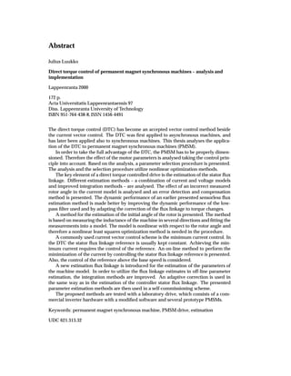
Some examples of these new industrial PMSMs developed at LUT are shown in Fig.
1.1. These 20-pole rotors have a varying air gap in order to get a sinusoidal flux den-
sity distribution created by the permanent magnets. This way the torque created by
sinusoidal currents contains as little ripple as possible. Also the cogging torque, often
regarded as a disadvantage of PMSMs, is reduced to minimum.
This thesis has its emphasis on the control of PMSMs of industrial type.
(a) Rotor 1: One magnet per pole (b) Rotor 2: Two magnets per pole
Figure 1.1: Industrial PMSM rotor constructions. Both rotors have 20 poles and the air gap is varied in
order to get a sinusoidal flux density distribution created by the permanent magnets.
15. 1.2 Fundamentals of the control principles 3
1.2 Fundamentals of the control principles
1.2.1 Current vector control
The earliest vector control principles for AC permanent magnet synchronous machines
resembled the control of a fully compensated DC machine. The idea was to control
the current of the machine in space quadrature with the magnetic flux created by the
permanent magnets. The torque is then directly proportional to the product of the flux
linkage created by the magnets and the current. In an AC machine the rotation of the
rotor demands that the flux must rotate at a certain frequency. If the current is then con-
trolled in space quadrature with the flux, the current must be an AC current in contrast
with the DC current of a DC machine.
The mathematical modelling of an AC synchronous machine is most conveniently
done using a coordinate system, which rotates synchronously with the magnetic axis
of the rotor, i.e. with the rotor. The x-axis of this coordinate system is called the direct
axis (usually denoted as ’d’) and the y-axis is the quadrature axis (denoted as ’q’). The
magnet flux lies on the d-axis and if the current is controlled in space quadrature with
the magnet flux it is aligned with the q-axis. This gives a commonly used name for this
type of the control, id 0 –control.
Unfortunately id 0 –control does not suite well to all permanent magnet machines.
The problem is that the air-gap flux is affected by the flux created by the current and the
inductance of the machine. This is called the armature reaction. Furthermore if the
magnetic circuit of the machine is not symmetrical in the direction of d- and q-axes, the
difference in the reluctance can be utilized in the torque production. If the direct axis
current is zero, this reluctance torque is also zero.
Different d- and q-axis inductances are a result of different d- and q-axis flux paths. If
the magnets are mounted on the rotor surface both the d-axis and the q-axis fluxes must
go through the magnet. The relative permeability of permanent magnets is usually near
unity, which means that permanent magnets are like air in the magnetic circuit. The
so called effective air-gap is therefore very large and the inductances due to the large
air-gap are quite low and nearly equal in d- and q-axes. If the magnets are mounted
in slots inside the rotor, the magnet flux paths are quite different. All the flux does not
have to go through the magnet and a considerable difference between the d-axis and
the q-axis inductances is possible. Since the q-axis flux does not necessarily go through
the magnet, usually the q-axis inductance is bigger than the d-axis inductance. This is
different from the separately excited synchronous machine where the d-axis inductance
is bigger.
The reluctance torque resulting in the inductance difference can and should be uti-
lized in the control. Analytical expressions for current references which maximize the
ratio of the torque and the current were first formulated by Jahns et al. (1986). This kind
of control is generally called the maximum torque per ampere control or minimum current
control.
In this thesis a term current vector control is used for all control methods, which con-
trol the torque via controlling the currents. Fig. 1.2 presents a principle block diagram of
the current vector control of PMSMs. The control system consists of separate controllers
for the torque and the current. Measurement or estimation of the rotor angle is needed
in the transformation of the d- and q-axis current components into fixed coordinate sys-
tem.
16. 4 Introduction
Rectifier Inverter PMSM
sA
sC
sB
is
Current
control
isb
isa
isc
£
i£
£
£
£
id «
£
te Torque Rotor to 2-phase to
control stator 3-phase
£ transformation
iq i£
¬
r
Figure 1.2: A principle block diagram of the current vector control of PMSMs
1.2.2 Direct torque control
A new kind of AC motor control was suggested by Takahashi and Noguchi (1986). Their
idea was to control the stator flux linkage and the torque directly, not via controlling the
stator current. This was accomplished by controlling the power switches directly using
the outputs of hysteresis comparators for the torque and the modulus of the stator flux
linkage and selecting an appropriate voltage vector from a predefined switching table.
The table was called the “optimum switching table”. A modification of the original control
diagram is presented in Fig. 1.3. In the original form the measurement of the rotor angle
was not used.
Almost simultaneously a same kind of control was proposed by Depenbrock (1987)
(appeared also in Depenbrock, 1988). At first, Takahashi and Noguchi did not give any
name to their new control principle. In a later paper by Takahashi and Ohmori (1987) the
control system was named the direct torque control, DTC. Depenbrock called his control
method Direct Self Control, DSC. Right after the papers by Takahashi and Noguchi and
Depenbrock only a few papers were published on the subject. After the introduction
of the first industrial application of the DTC (Tiitinen et al., 1995) the number of papers
on the DTC has grown tremendously. Quite a few of them are on different aspects
of the DTC for asynchronous motors (see e.g. Griva et al., 1998; Damiano et al., 1999),
but in recent years there has been also interest to apply the DTC to permanent magnet
synchronous motors. There are papers e.g. by Zolghadri et al. (1997), Zolghadri and
Roye (1998), Zhong et al. (1997), Rahman et al. (1998a) and Rahman et al. (1998b).
Today, the DTC has become an accepted control method beside the field oriented
control. Even a text book has been published by Vas (1998), which concentrates on the
DTC and other sensorless control methods.
17. 1.2 Fundamentals of the control principles 5
PMSM
sA, SB, SC
is
Switching table r
us 3 2
£
· Voltage Current
s
model model
·
su si
£
te s
te s
correction
Figure 1.3: A block diagram of the control principle originally presented by Takahashi and Noguchi (1986).
A modification has been made to the flux linkage calculation by adding the traditional current
model to improve the calculation of the flux linkage especially at low speeds.
18. 6 Introduction
1.2.3 Comparison of control principles
In many references the control of a PMSM is separated from the control of other types
of AC machines. However, it can be stated that a PMSM is a regular rotating field AC
machine and the control is similar to that of other types of AC machines. The control
principle which is considered in this thesis, the direct torque control, makes this state-
ment even more justified. A PMSM can be thought as a synchronous machine with
constant excitation current. The following differences may nevertheless be noticed:
• The stator inductance of a PMSM may be quite low
• The quadrature axis inductance is bigger than or equal to the direct axis induc-
tance
• There are usually no damper windings
• The power factor, although controllable, does not directly describe the relationship
between the torque and the stator current (compare this with a separately excited
field winding where the power factor can be controlled to unity by controlling the
field current)
• There are no typical PM machines. The inductances are quite different from ma-
chine to machine from negligible to above 1.0 pu. Compare this to induction ma-
chines, where the stator inductance is always above 1.0 pu.
1.3 Outline of the thesis
The purpose of this thesis is to present an analysis and an implementation of a direct
torque controlled permanent magnet synchronous motor or generator drive. Since there
is not usually much difference between a motor or a generator drive, a term machine is
used to refer to both.
In order to take the full advantage of using the direct torque control, first an analysis
of the effect of machine parameters on the performance of the drive is presented. Based
on the analysis, a design procedure is developed for selecting the parameters of a per-
manent magnet synchronous machine especially for direct torque controlled drives. The
requirements, which the direct torque control sets to the selection, are also compared to
the requirements of the commonly used minimum current vector control.
The second main topic is the implementation of the direct torque controlled drive.
The purpose is to implement both a position sensored and a position sensorless drive.
The drive should include an accurate estimation of the stator flux linkage, the control of
the reference of the stator flux linkage and the limitation of the load angle. All of these
should work both with and without position measurement. Not including the lowest
speeds, the performance of the position sensorless estimation of the stator flux linkage
should be as good as that of the position sensored one. The estimation of the stator
flux linkage should also include the estimation of the initial angle of the rotor, since
when starting a synchronous machine, the initial value of the stator flux linkage must
be known. If possible, the position sensored version should require only an incremental
encoder, not an absolute one. This is a question of reliability and cost. To get rid off the
absolute encoder, the initial angle estimation method should also include an elimination
method for the error of the initialization of the angle calculated from the incremental
encoder. All of these issues are considered in this thesis.
19. 1.3 Outline of the thesis 7
The control system should also be able to estimate the parameters of the machine
model itself. The estimation can be performed either on-line or off-line. The off-line
methods are usually easier to implement and the estimation can take place during the
commissioning of the drive. Most of the parameters do not change during the operation
of the drive, and therefore on-line estimation is rarely needed. The estimation methods,
which will be considered in this thesis, are off-line methods. These methods should
work both with and without position measurement and they should utilize the existing
stator flux estimation of the direct torque control as far as possible.
The contents are divided into seven chapters. Beside this introductory chapter, the
following chapters are presented:
Chapter 2 introduces the reader to the mathematical model used. The purpose is to
give an introduction on the space vector theory, which is used throughout the
thesis.
Chapter 3 presents an analysis of the effect of the machine parameters on the drive
performance. Based on the analysis, the selection of the parameters of a PMSM
for variable speed drives is examined. The selection is based on the optimization
of the nominal torque or the nominal current. Special attention is paid to setting
the constraints properly according to the control principle. The solution technique
is new compared to methods presented in literature. The solution procedure is
implemented as an interactive computer program.
Chapter 4 deals with the direct torque control of a PMSM. The chapter analyses the
estimation of the stator flux linkage used in the selection of voltage vectors, the
initial angle of the PMSM and the control of the flux linkage reference. Also, the
limitation of the load angle is considered.
Chapter 5 presents an analysis of the estimation of the parameters of the motor model.
The chapter analyses first the methods to estimate the flux linkage to be used in
the estimation of the parameters. Then the estimation of various parameters is
presented using the analysed estimation methods. The presentation is concluded
with a self-tuning procedure which uses the presented methods in the commis-
sioning stage of a direct torque controlled PMSM drive.
Chapter 6 presents the experimental verification of the presented methods with a labo-
ratory test drive. Some of the methods were tested with many motors and invert-
ers to show that the methods are applicable for motors with different parameters.
Chapter 7 presents conclusions and some suggestions on future work.
Simulations are presented in all the chapters to illustrate the behaviour of presented
methods.
20.
21. Chapter 2
Modelling of permanent magnet
synchronous machines
Ì × ÔØ Ö Ú × Ò ÒØÖÓ Ù Ø ÓÒ ØÓ Ø ×Ô Ú ØÓÖ Ø ÓÖÝ Ò Ø× ÔÔÐ Ø ÓÒ ÓÒ ÑÓ ÐÐ Ò
Ó Ô ÖÑ Ò ÒØ Ñ Ò Ø ×ÝÒ ÖÓÒÓÙ× Ñ Ò ×º Ð×Ó¸ Ø Ù× Ó Ô Ö¹ÙÒ Ø Ú ÐÙ ÕÙ Ø ÓÒ× ×
ÔÖ × ÒØ º
2.1 Space vectors
In the theory and analysis of AC systems it is common to express the quantities which in
general are functions of time as complex numbers. E.g. a sinusoidally varying current
i(t) is expressed as
¡
i(t) i cos · j sin ie j (2.1)
where i is the peak value of the current and t ·
is the phase angle of the cur-
rent. Either of the components can be selected to represent the instantaneous value of
the current, although usually the imaginary part is selected, i.e. i(t) Im i i sin .
In a symmetrical p phase system the phases are displaced by an angle 2 p. By select-
ing the real part of the current to represent the instantaneous value of the current, the
instantaneous values of the phase currents of a three-phase system may be expressed as
ia (t) i cos ( t · ) (2.2)
¡
ib (t) i cos t 2 3· (2.3)
¡
ic (t) i cos t 4 3· (2.4)
Let us consider a stator of an AC machine which has a three-phase winding. For sim-
plicity let us assume that each winding consists of a single coil which creates a sinu-
soidally distributed magneto-motive-force (mmf for short), i.e. the spatial harmonics
are neglected. The mmf distribution f s created by the three-phase currents is then
¢
fs ( t) Nse ia (t) cos · ib(t) cos 2 3
¡
· ic (t) cos 4 3
¡£
(2.5)
where is the angle from the reference axis, and Nse is the equivalent number of turns.
The equation may also be expressed as
Ò ¢ £ Ó
fs ( t)
1
c
Nse Re c ia (t) · a ib(t) · a2 ic (t) e j (2.6)
22. 10 Modelling of permanent magnet synchronous machines
where a is an operator defined as
a e j2 3
(2.7)
Eq. (2.6) contains the definition of the space vector of the stator current
¢
is (t) c ia (t) · a ib (t) · a2 ic (t)£ i s e j «s (2.8)
where c is a scaling constant. Similarly space vectors for voltage and flux linkage may
be expressed
¢ £
(t) c · a b(t) · a2 c (t)
a (t) (2.9)
s
¢ £
us (t) c ua (t) · a ub (t) · a2 uc (t) (2.10)
c may be selected arbitrarily. The selection, however, affects for example the equations
of power and torque. The three-phase power P may be expressed as
3
P 3Re UI £ ui cos ³ (2.11)
2
where U is the phasor of the phase voltage, I £ is the complex conjugate of the phasor of
the phase current and u and i are the peak values of the phase quantities. As space vec-
tors are used to represent the whole three-phase system, the power should be expressed
with Re ui£ without the number of phases as a factor:
P Re ui£ c2 ui cos ³ (2.12)
Ô
If we select c 3 2 these two equations of the power are equal. This gives the power-
invariant form of the space vectors. The classical non-power-invariant form is obtained by
setting c 2 3. The non-power-invariant form will be used in this thesis except in the
per-unit valued equations (see Section 2.4).
By making an assumption that there are no zero sequence currents the following
relation is written
ia (t) · ib (t) · ic (t) 0 (2.13)
One of the currents can be eliminated and therefore one degree of freedom is reduced
and the space vectors may be expressed by an equivalent two-phase system, which
consists of real and imaginary parts
is (t) Re is · jIm is is« (t) · jis¬ (t) (2.14)
For a more complete presentation of space vectors applied to electrical machines see e.g.
(Vas, 1992).
2.2 Voltage and flux linkage equations
In order to obtain the mathematical model of a permanent magnet synchronous ma-
chine let us first consider a simplified model. The stator voltage us consists of a resistive
s
part created by the Ohmic loss of the stator resistance Rs and a part which depends on
the rate of change of the stator flux linkage ss
s
d
us
s Rs i s
s · dt
s
(2.15)
23. 2.2 Voltage and flux linkage equations 11
where the superscript ’s’ expresses that the quantities are expressed in a coordinate
system which is bound to stator, i.e. it is stationary in time.
The flux linking the stator winding consists of the contribution of the flux created
in the stator self inductance and the flux created by the permanent magnets. The flux
linkage created by the permanent magnets depends on the angle of the rotor r from a
reference axis. Therefore the stator flux linkage may be expressed as
s
s
Ls is
s · PM e
j r
(2.16)
Substituting this into (2.15) gives
¡
d Ls i s
s
us Rs i s
s · dt
s
·j r PM e
j r
(2.17)
Let us define the space vectors of the stator voltage and the stator current expressed in
the coordinate system bound to rotor
ur
s u s e j
s
r
(2.18)
ir
s i s e j
s
r
(2.19)
The voltage equation is transformed to
¡
d Ls i r ¡
r
us Rs i r
s · dt
s
·j r Ls i r
s · PM (2.20)
· ·
Let ur usd jusq and ir isd jisq . The following equations are obtained by separating
s s
the real and imaginary parts from the above equation
usd Rs isd · d (Ls isd )
dt
r Ls isq Rs isd · ddtsd r sq (2.21)
¡
usq Rs isq ·d Ls isq
dt
· r (Ls isd · PM ) Rs isq · ddtsq · r sd (2.22)
The first parts of these equations define the direct and the quadrature axis components of
a non-salient pole permanent magnet synchronous machine without damper windings.
The last parts of the equations also apply to salient-pole machines with damper wind-
ings. In salient-pole machines the magnetic circuit is such that the reluctance along the
direct axis is different than along the quadrature axis resulting in different inductances
in direct and quadrature directions. In general the stator and damper winding flux
linkages are defined as
sd Lsd isd · Lmd iD · PM (2.23)
sq Lsq isq · Lmq iQ (2.24)
D Lmd isd · LD iD · PM (2.25)
Q Lmq isq · LQ iQ (2.26)
where sd and sq are the direct and quadrature axis components of the stator flux link-
age and D and Q the components of the damper winding flux linkage. The voltage
equations of the short-circuited damper windings are
0 RD iD · ddtD (2.27)
0 RQ iQ · ddtQ (2.28)
24. 12 Modelling of permanent magnet synchronous machines
where RD and RQ are the direct and quadrature axis components of the resistance of
the damper winding. Now that all the quantities have been defined we can present the
equivalent circuit of a PMSM. The equivalent circuit depicted in Fig. 2.1 is divided into
d- and q-axes like the equations describing the quantities.
isd Rs Ls iD
imd
RD if
usd Lmd
LD
sq
(a) d-axis
isq Rs Ls iQ
imq
RQ
usq Lmq
LQ
sd
(b) q-axis
Figure 2.1: The equivalent circuits of a PMSM.
It is often useful to express the flux linkages in matrix form
¾ ¿ ¾ ¿¾ ¿ ¾ ¿
sd Lsd 0 Lmd 0 isd 1
sq
D
0
Lmd
Lsq
0
0
LD
Lmq
0
isq
iD
· PM
0
1
(2.29)
Q 0 Lmq 0 LQ iQ 0
Expressing the voltage equation of a salient-pole PMSM with one complex equation
25. 2.3 Equations of the torque 13
(like (2.20)) is not unfortunately possible. A similar equation can, however, be for-
mulated using matrices. Let us think of (2.29) in steady state. We may leave out the
components that are zero and rewrite the equation as follows
sd
sq
Lsd
0
0
Lsq
isd
isq
· PM
1
0
(2.30)
Using matrix notation this is expressed as
r
s
r
Lis · PM (2.31)
r T r
where s [ sd sq ] , is [isd isq ]T , PM PM [1 0]T and
Lsd 0
L (2.32)
0 Lsq
Let us define also ur
s [usd usq ]T . Then the voltage equation may be expressed as
r
ur
s
r
Rs i s · ddt s · rJ
r
s (2.33)
where J is a matrix corresponding to the imaginary unit j and it is defined as
J
0 1 (2.34)
1 0
J has some similar properties with j. E.g. similarly like j2 1:
JJ I (2.35)
where I is an identity matrix. The complex vector rotator e j may also be expressed
with J. The Euler’s equation e j cos ·
j sin can be extended for matrices:
eJ I cos · J sin (2.36)
It is also useful to notice that the matrix inverse of e J is e J and vice versa:
1
eJ e J (2.37)
Extended Euler’s equation (2.36) can easily be proofed with series expansion of e J . The
stator flux linkage (Eq. (2.31)) can be transformed to stator reference frame by
s
s eJ r
s
r
e J Lis · eJ PM e J Le J is
s
· eJ PM (2.38)
It should be noted that when dealing with matrices the order of the matrix product is of
importance. E.g.
e J L 1 e J e J e J L 1 L 1 (2.39)
2.3 Equations of the torque
If only the fundamental of the stator-mmf is considered the torque te of an AC machine
is expressed as a vector, which is for the non-power-invariant form
te
3
2
pN s
¢ is (2.40)
26. 14 Modelling of permanent magnet synchronous machines
where pN is the number of pole pairs. If the flux linkage and the stator current are
considered as vectors in xy-plane
s
· s¬ j¯
s« i
¯ (2.41)
is is« i · is¬ j
¯ ¯ (2.42)
then the torque is perpendicular to xy-plane, i.e.
3 ¡¯
te
2
pN s« is¬ s¬ is« k (2.43)
Usually, though, s and is are considered as complex valued vectors and then the z-
axis has no meaning. We can therefore usually consider the torque as a scalar t e , which
means that we only take the z-component of the cross product. Mathematically such an
¯
operation is denoted as a scalar projection of the torque t on the unit vector k e
3 ¡
te ¡ ¯
te k
2
pN s« is¬ s¬ is« (2.44)
The cross product in the equation of the torque reveals that the equation is independent
on the coordinate system used – the cross product depends only on the angle between
the vectors. Therefore the torque may be calculated either from the quantities in the
stator coordinates or in the rotor coordinates – or in any coordinates. In the rotor coor-
dinates the equation of the torque becomes
3 ¡
te
2
pN sd isq sq isd (2.45)
3 ¢ ¡ £
2
pN PM isq Lsq Lsd isd isq (2.46)
It is often useful to express the reluctance torque differently. Let us define a parameter
called the saliency ratio
Lsq Lsd
(2.47)
Lsq
The inductances can then be expressed as
Lsd Lsq (1 ) (2.48)
Lsd
Lsq
1 (2.49)
The equation of the torque is transformed to
3 ¡
te
2
pN PM isq Lsq isd isq (2.50)
The advantage of this equation is that it is easier to analyse the effect of different induc-
tances on the torque than with the original one. The saliency ratio describes the possi-
ble inductance range better than the absolute difference between inductances, L sq Lsd .
2.4 Per-unit valued equations
It is often convenient to express the quantities of an AC system, such as a motor, in di-
mensionless form, in so-called per-unit values. This way motors of different dimensions
can easily be compared with each other.
29. Chapter 3
Selection of the parameters of a
PMSM
ÁÒ Ø × ÔØ Ö¸ Ø Ø Ó Ø ÑÓØÓÖ Ô Ö Ñ Ø Ö× ÓÒ Ø Ô Ö ÓÖÑ Ò Ó Ø Ö Ú × Ò ÐÝ× º
× ÓÒ Ø Ò ÐÝ× ×¸ Ò Û Ñ Ø Ó Ó × Ð Ø Ò Ø Ô Ö Ñ Ø Ö× × ÔÖ × ÒØ º Ì ÔÖÓ ÙÖ
× × ÓÒ Ñ Ü Ñ Þ Ò Ø ÔÓÛ Ö ØÓÖ Ø Ø ÒÓÑ Ò Ð ÐÓ ÓÒ× Ö Ò Ø ÓÒØÖÓÐ ÔÖ Ò ÔÐ
Ò Ø Ö ÕÙ Ö Ñ ÒØ× Ó Ø ÔÔÐ Ø ÓÒº
3.1 Introduction
The designing of PM-machines has not matured yet to a degree which e.g. the designing
of induction machines has. During the recent years there has been a considerable in-
crease of interest in using PM-machines in applications where previously asynchronous
machines have been used. Traditionally PM-machines have been used in low-power
servo drives, but with the recent development in both permanent magnets and power
electronics also medium and large power drives are gaining more interest (see e.g. Rosu
et al., 1998). The suitability of a permanent magnet motor to a particular application is,
however, dependent on the motor design. If for example large field-weakening range is
needed, the motor has to have a large enough direct axis inductance. This in turn de-
creases the torque capability in the nominal flux area. Selecting the parameters to fulfill
the requirements of the application is clearly an optimization problem.
The parameters of the motor also affect the control. E.g. the traditional i sd 0-control
is not very usable if the armature reaction is big, i.e. the inductances of the machine are
considerable. As the torque is increased, keeping the direct-axis current zero results in
increase of the modulus of the stator flux linkage. This in turn results in increased iron
losses. Increased flux linkage also increases the stator voltage and therefore with the
same motor the maximum speed with isd 0 is lower than e.g. with constant s .
The selection of the motor parameters has been analysed e.g. by Schiferl and Lipo
(1990), Morimoto et al. (1990), Ådnanes (1991), Morimoto et al. (1994a) and Bianchi and
Bolognani (1997). All of these papers examine the problem using a per-unit system
which differs from the usual per-unit system described in Section 2.4. The main differ-
ence in that per-unit system is that the base current Ib is defined as
Ô Õ
Ib 2IN 2
Idopt · Iqopt
2 (3.1)
30. 18 Selection of the parameters of a PMSM
where Idopt and Iqopt are the current components giving the minimum current. These
currents are functions of all the parameters PM , Lsd and Lsq (this will be seen in Eqs.
(3.22) and (3.23)). In consequence one of the three parameters is fixed if the other two
are changed. Also, the base current changes as the parameters change. The drawback
with this is that it is hard to analyse which would be the optimum values of Lsd and Lsq
independent on each other. This per-unit system guarantees only that 1 pu. values for
stator current, voltage and flux linkage at one per-unit speed give a maximum torque
to current ratio. The torque obtained this way does not keep constant as the parameters
are changed, so the per-unit system selection cannot be justified with an equal power
between different parameters. Since the voltage limitation is not used when obtaining
the equations for Idopt and Iqopt there is no guarantee that the obtained parameters give
the maximum torque which could be obtained with the available current and voltage.
Furthermore, the control principle is tied to minimum current control.
Thelin and Nee (1998) make some suggestions regarding the pole-number of inverter-
fed PMSMs. Their only selection criterion was the efficiency of the motor. The selection
of the pole-number is not considered in this thesis. However, it should be noted that
the pole number has got a big influence on the freedom of parameter selection. For
example, if the pole-number is big, the magnetizing inductance tends to become small
compared to the stator leakage inductance. Therefore obtaining a large inductance ratio
is difficult. The equation of the magnetizing inductance Lm shows that the inductance
is inversely proportional to the number of pole pairs pN (Vogt, 1996)
3 2 1 D
Lm 0 (N 1 ) li (3.2)
p 2 Æi
N
where li is the length of the active parts, D is the air-gap diameter and Æ i is the air-gap.
In this chapter a new solution technique is presented for the selection of PMSM’s
parameters. The solution is based on mathematical optimization with appropriate con-
straints. The target function of the optimization is the nominal torque with the induc-
tances and the permanent magnet’s flux linkage as variables. By solving the optimiza-
tion problem with inductances as parameters we can analyse their effect on the nominal
torque and, based on that, select the inductances and permanent magnet’s flux linkage.
The examination is divided so that first Section 3.2 analyses what affects the torque
and power behaviour of a PMSM. Section 3.3 considers then what kind of constraints
the application sets for the parameter selection. Section 3.4 then presents the basic op-
timization scheme and its results for different control principles. Section 3.5 brings one
optimization criterion more, the maximum torque, to the problem. In Section 3.6 the
field-weakening area is considered. Finally, Section 3.7 gathers all the constraints and
presents a parameter selection procedure. The selection procedure is implemented as
an interactive computer program.
3.2 The torque and power performance of a PMSM
In order to select the parameters of a PMSM, one must study the torque behaviour of
a PMSM in detail. The equation of the torque was given in Eq. (2.46), which is shown
here again, but this time in the per-unit scale
¡
te sd isq sq isd PM isq Lsq Lsd isd isq
31. 3.2 The torque and power performance of a PMSM 19
In isd , isq plane this is an equation of a hyperbola
te
¡
PM Lsd
isq (3.3)
Lsq isd
The hyperbolas have asymptotes
isq 0 (3.4)
PM
isd
Lsq Lsd (3.5)
The latter is obtained by solving isd from Eq. (3.3) as i sq . The hyperbolas are il- ½
lustrated in Fig. 3.1. Each hyperbola forms a so-called constant torque hyperbola. This
means that the same torque is produced by all the different combinations of isd and isq
forming the hyperbola. Therefore there is a great freedom in selecting the currents pro-
ducing the wanted torque. Moving along the hyperbola changes the modulus of the
stator flux linkage and thus the needed voltage. On the other hand at the same time the
modulus of the stator current is changed. It is obvious that there exists a minimum for
the stator current for each given torque. The minimum can be used as a basis of current
references in current vector control.
ten 1
ten 2 3
iqn
ten 3
ten 1
ten 2
ten 3 2
1
0
-3 -2 -1 0 1 2 3
-1 idn
-2
-3
Figure 3.1: Constant torque hyperbolas. A normalization introduced by Jahns et al. (1986) is used. The
normalization is described later.
Let us examine the minimum in detail. The modulus of the stator current is ex-
pressed as
is 2 2
isd · isq
2
(3.6)
32. 20 Selection of the parameters of a PMSM
This is clearly an equation of a circle in isd , isq plane. Moving on a circle in isd , isq plane
keeps the current constant but the torque is changed as the observation point moves
from one constant torque hyperbola to another. At a given torque the minimum of
the stator current is obtained when the tangents of the torque hyperbola and the stator
current circle are parallel. Let us derive equations for these optimum i sd and isq , which
gives us equations for the current references which minimize the stator current at a
given torque.
Let us introduce the following normalizations (Jahns et al., 1986)
ten te teb (3.7)
iqn isq ib (3.8)
idn isd ib (3.9)
with the base values
PM
ib
Lsq Lsd (3.10)
teb PM ib (3.11)
The above base values are defined so that the normalization is made from the usual
per-unit valued equations (this is different in Jahns et al., 1986). The normalized torque
ten is then obtained from the per-unit torque te as follows
¡ 2
te PM isq Lsd isdisq
Lsq : teb
Lsq
PM
Lsd
¸ te
teb
isq
PM
· Lsd Lsq i i
2
PM
sq sd
Lsq Lsd Lsq Lsd
¸ ten isq
PM
1 · Lsd Lsq isd
Lsq Lsd PM
¸ ten isq
ib
1 iisd
b
Finally
ten iqn (1 idn ) (3.12)
Now, iqn is eliminated
ten
iqn
1 idn (3.13)
The squared modulus of the normalized stator current is then
2
in 2 2
idn · iqn
2 2
idn · ten
1 idn
(3.14)
The minimum of the current in at the given torque ten is obtained by differentiating Eq.
(3.14) with respect to i dn and setting the derivative zero:
d in 2 2
2idn · 2 ten 3 0
didn (1 idn )
¸ t2
en idn (idn 1)3 (3.15)
33. 3.2 The torque and power performance of a PMSM 21
Eq. (3.15) forms the basis for the direct axis current reference. The equation for quadra-
ture axis current reference is obtained similarly by eliminating isd from Eq. (3.12). The
following equation is obtained from the derivative’s zero condition
t2
en teniqn iqn
4
0 (3.16)
An explicit equation for iqn is obtained by solving ten as a root of the second order equa-
tion
Õ
ten
iqn
2
1 ¦ 1 · 4iqn
2 (3.17)
Since the expression under the square root is always greater than one, we know that
only the ’+’-sign is allowed. Therefore the equation for iqn is
Õ
ten
iqn
2
1 · 1 · 4iqn
2 (3.18)
Eqs. (3.15) and (3.18) were first presented by Jahns et al. (1986). Solving both i dn and iqn
requires iteration or the nonlinear relationship between the torque ten and the currents
must be saved in a look-up table. A simplification can, however, be made. Solving i dn
from (3.12) gives
idn 1 iten (3.19)
qn
From (3.18)
Õ
ten
iqn
1
2
1 · 1 · 4iqn
2 (3.20)
Combining (3.19) and (3.20) gives a solution to i dn as a function of iqn
Õ
idn
1
2
1 1 · 4iqn
2 (3.21)
The return back to usual per-unit system is obtained as follows. Substitute (3.7) and
(3.8) into (3.18)
¾ Ú ¿
Ù ¡2
Ù 2 L L
te
PM isq Ø
1· 1·4
isq sq sd
(3.22)
2 2
PM
Õ
PM
¡ 1 · 4iqn
2
isd ib idn
2 Lsq Lsd 1
Ú
Ù
Ù 2
PM
¡ Ø PM
· isq
Lsd¡2
2
2 Lsq Lsd 4 Lsq
(3.23)
The reference for quadrature axis current i sq is found as a solution of Eq. (3.22) and the
direct axis reference from Eq. (3.23). It should be noted that if L sd Lsq the latter of
these equations is not defined. Should this be the case the references are simply
te
isq (3.24)
PM
isd 0 (3.25)