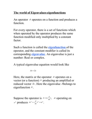
1. The world of Eigenvalues-eigenfunctions
An operator A operates on a function and produces a
function.
For every operator, there is a set of functions which
when operated by the operator produces the same
function modified only multiplied by a constant
factor.
Such a function is called the eigenfunction of the
operator, and the constant modifier is called its
corresponding eigenvalue. An eigenvalue is just a
number: Real or complex.
A typical eigenvalue equation would look like
Ax = λ x
Here, the matrix or the operator A operates on a
vector (or a function) x producing an amplified or
reduced vector λx . Here the eigenvalue λbelongs to
eigenfunction x .
d
Suppose the operator is A = ( x dx ) . A operating on
d n
x n produces Ax = x x = nx .
n n
dx

2. Therefore, the operator A has an eigenvalue n
corresponding to eigenfunction x n .
1. Eigenfunctions are not unique.
Suppose Ax = λ x . Define, another vector z = cx , where
c is a constant.
Now, Az = Acx = cAx = cλ x = λ cx = λ z
Therefore, z is also an e-function (eigenfunction)
of A.
2. If Ax = λ x is an eigenvalue equation (and we
assume that x is not a zero vector), then
Ax = λx ⇔ (A - λI)x = 0 ⇐⇒ det(A - λI) = 0
This leads to a characteristic polynomial in λ:
p A = det( A − λ I )
λ is an e-value of A only if pA = 0.
3. Spectrum of an operator A is σ( A ) : set of all its
e-values.
4. Spectral radius of an operator A is
ρ ( A ) = max | λ |
λ∈σ ( A ) = 1maxn | λi |
≤i ≤
5. Computation of spectrum and spectral radius:

3. 2 −1
Let A = 2 5  be the matrix and we want to
 
compute its eigenvalues and eigenfunctions. Its
characteristic equation (CE) is:
2 − λ −1 
det  = 0 ⇐⇒ (2 - λ )(5 - λ ) + 2 = 0
 2 5 − λ

This gives λ2 − 7λ + 12 = 0 ⇐ ⇒ ( λ − 3 )( λ − 4 ) = 0
Therefore, A has two eigenvalues: 3 and 4.
x 
Let the eigenfunction be the vector x =  1
 x2 
corresponding to e-value 3. Then
 2 − 1  x1   x1   3 x1 
 2 5   x  = 3 x  =  3 x 
  2   2   2 
Therefore, we have 2 x1 − x2 = 3x1 yielding
x1 = − x2 . Also, we get 2 x1 + 5 x2 = 3 x2 which gives us no new
result. Therefore, we can arbitrarily take the
1 
following solution: e1 = −1 corresponding to e-value 3
 
for the matrix A.

4. Similarly, for e-value of 4, the eigenfunction appears
1 
to be e2 = − 2 .
 
6. Faddeev-Leverrier Method to get characteristic
polynomial.
Define a sequence of matrices P = A, p1 = trace( P )
1 1
1
P2 = A[ P − p1I ] , p2 = trace( P2 )
1
2
1
P3 = A[ P2 − p2 I ] , p3 = trace( P3 )
3
…
…
1
Pn = A[ Pn −1 − pn −1I ] , p n = trace( Pn )
n
Then the characteristic polynomial P( λ ) is
[
P( λ ) = ( −1 )n λn − p1λn −1 − p2 λn − 2 − ... − pn ]
12 6 − 6
 6 16 2 
e.g. A=
 
− 6 2
 16 

Define P = A, p1 = trace( A ) = 12 + 16 + 16 = 44
1
P2 = A( P − p1I ) =
1
12 6 − 6− 32 6 −6 
 6 16 2  6 − 28 2 
  
− 6 2
 16  − 6
 2 − 28

− 312 −108 108 
= −108 − 408 − 60 , p 2 = −564
 
 108
 − 60 − 408


5. And one proceeds this way to get p3 = 1728
The CA polynomial = ( −1 )3 [λ3 − 44λ2 + 564λ −1728]
The eigenvalues are next found solving
[λ3 − 44λ2 + 564λ −1728] = 0
7. More facts about eigenvalues.
Assume Ax = λ x . Therefore, λ is the eigenvalue of
A with eigenvector x .
a. A−1 has the same eigenvector as A and the
corresponding eigenvalue is λ−1 .
b. An has the same eigenvector as A with the
eigenvalue λn .
c. ( A + µI ) has the same eigenvector as A with the
eigenvalue ( λ + µ ) .
d. If A is symmetric, all its eigenvalues are real.
e. If P is an invertible matrix then P −1 AP has the
same eigenvalues as A .
Proof of e.

6. Suppose, the eigenfunction of P −1 AP is y with
eigenvalue k .
Then,
P − APy = ky
1
⇐⇒ APy = Pky = kPy
Therefore, Py = x and k must be equal to λ. Therefore
the eigenvalues of A and P −1 AP are identical and the
eigenvector of one is a linear mapping of the other
one.
If the eigenvalues of A , λ1 ,λ2 ,...,λn are all distinct
then there exists a similarity transformation such that
λ1 0 0 .. 0 
0 λ 0 .. 0 
 2 
−1
P AP = D =  0 0 λ3 .. 0 
 .. .. .. .. 0 
 

0 0 0 .. λn 

Let the eigenvectors of A be x ( 1 ) , x ( 2 ) ,..., x ( i ) ,...x ( n )
such that we have Ax( i ) = λi x( i )
Then the matrix P = [ x( 1 ) , x( 2 ) ,..., x( n ) ]
Then AP = [ Ax( 1 ) , Ax( 2 ) ,..., Ax( n ) ]
[
= λ1 x( 1 ) ,λ2 x( 2 ) ,..., λn x( n ) ]
[ ][
= x ( 1 ) , x ( 2 ) ,..., x ( n ) λ1e( 1 ) ,λ 2 e( 2 ) ,..., λn e( n ) ]
= PD
Therefore, P −1 AP = D
Also, note the following. If A is symmetric, then

7. . So, we can normalize each
( x ( i ) )t x ( j)
= 0 , ∀i ≠ j
(i )
x (i)
eigenvector and obtain u = x so that the (i )
matrix Q = [u ( 1 ) ,u ( 2 ) ,...,u ( n ) ] would be an orthogonal matrix.
i.e. Q AQ = Dt
Matrix-norm.
Computationally, the l 2 -norm of a matrix is
determined as
l 2 -norm of [
A =|| A ||2 = ρ( At A ) ]1 / 2
1 1 0
e.g. A = 1 2 1
 
−1
 1 2

1 1 −1 1 1 0  3 2 −1
Then A A = 1
t
2 1  1 2 1 =  2 6 4
    
0
 1 2 −1
 1 2 −1
  4 5
The eigenvalues are:
λ1 = 0, λ2 = 7 + 7 , λ3 = 7 − 7
Therefore, A2 = ρ( At A ) = 7 + 7 ≈ 3.106
A ∞ = max ∑ aij
The l∞norm is defined as 1≤i ≤n j
1 1 0 
e.g. A =1 2 1 
 
−1
 1 − 4


8. 3 3
∑ a1 j = 1 + 1 + 0 = 2 , ∑ a2 j = 1 + 2 + 1 = 4
j =1 j =1
3
∑ a3 j = 6
j =1
Therefore, A ∞ = max( 2 ,4 ,6 ) = 6
In computational matrix algebra, we would often be
interested about situations when A k becomes small
(all the entrees become almost zero). In that case, A is
considered convergent.
is convergent if klim∞( A )ij = 0
k
i.e. A →
1 
 0
Example. Is A = 2 convergent?
1 1
 
4 2
1  1  1 
 4 0 8 0 16 0 
A2 =  A3 =  A4 = 
1 1 , 3 1 , 1 1 ,
     
 4 4 16 8   8 16 
It appears that
 1 
 2k 0
Ak = 
k 1
 
 2k + 1 2k 
 

9. 1
In the limit k → ∞,
2k
→0 . Therefore, A is a convergent
matrix.
Note the following equivalent results:
a. A is a convergent matrix
k
b1. klim∞ A 2 = 0
→
k
b2. klim∞ A ∞ = 0
→
c. ρ( A ) < 1
k
d. klim∞ A x = 0 ∀x
→
Condition number K( A ) of a non-singular matrix A
is computed as
K ( A ) = A . A -1
A matrix is well-behaved if its condition number is
close to 1. When K ( A ) of a matrix A is significantly
larger than 1, we call it an ill-behaved matrix.