This document provides an overview of exponential and logarithmic functions. It defines exponential functions as functions of the form f(x) = A*bx, where A and b are constants. Exponential functions model phenomena like radioactive decay and population growth. Logarithms are defined as the power to which a base number must be raised to equal the input value. Properties of logarithms include log(ab) = log(a) + log(b). Logarithms are useful for solving equations involving exponents. The derivatives of logarithmic and exponential functions are discussed but not derived until integration is covered.
1. CHAPTER 17: EXPONENTIAL AND LOGARITHM
FUNCTIONS
1. Exponential Functions
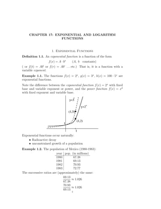
Definition 1.1. An exponential function is a function of the form
f (x) = A · bx (A, b constants)
t r
( or f (t) = Ab or f (r) = Ab . . . etc.) That is, it is a function with a
variable exponent.
Example 1.1. The functions f (x) = 2x , g(x) = 3x , h(x) = 100 · 5x are
exponential functions.
Note the difference between the exponential function f (x) = 2x with fixed
base and variable exponent or power, and the power function f (x) = x2
with fixed exponent and variable base.
Exponential functions occur naturally:
• Radioactive decay
• unconstrained growth of a population
Example 1.2. The population of Mexico (1980-1983):
year pop. (in millions)
1980 67.38
1981 69.13
1982 70.93
1983 72.77
The successsive ratios are (approximately) the same:
69.13
≈ 1.026
67.38
70.93
≈ 1.026
69.13
1
2. 2 First Science MATH1200 Calculus
In each year, the population increases by a factor of 1.026.
Let P (t) denote the population at time t (where t is the number of years
since 1980):
P (0) = 67.38 = P0
P (1) = 67.38 · (1.026)
P (2) = 67.38 · (1.026) · (1.026) = 67.38 · (1.026)2
P (3) = 67.38 · (1.026)3
.
.
.
P (t) = 67.38 · (1.026)t = P0 bt
Thus the estimated population in 1990 is P (10) = 67.38 · (1.026)10 ≈ 87.1
Note: If f (t) = Abt , we get exponential growth if b > 1 and we get expo-
nential decay if b < 1. (b is called the base of the exponential function.)
Example 1.3. Consider the exponential function f (t) = (1/2)t = 2−t :
This function exhibits exponential decay.
Example 1.4. For any given amount of radioactive potassium ( 44 K ),
19
the amount remaining one second later is 99.97%. Find a formula for the
amount at time t. (Let A0 be the amount at time 0).
3. First Science MATH1200 Calculus 3
Solution:
A(t) = amount at time t
A(0) = A0
A(1) = A0 · (0.9997)
.
.
.
A(t) = A0 · (0.9997)t
2. Half-Lives
Suppose that A(t) = A0 · bt with b < 1
(i.e., we have exponential decay).
Then there is a number h > 0 with
1
bh =
2
Thus, if t is any time, the amount at time t + h is
A(t + h) = A0 · bt+h
= A0 · b t · b h
1
= A0 b t
2
1
= A(t)
2
1
= of the amount at time t
2
The number h is called the half-life or 1/2-life of the process.
44
Example 2.1. The 1/2-life of 19 K is 22 mins.
Example 2.2. The 1/2-life of Carbon-14 is 5700 years.
A similar computation shows that if we have exponential growth
A(t) = A0 bt b>1
then bd = 2 for some d > 0.
This number d is called the doubling time for the process.
Example 2.3. The 1/2-life of carbon-14 is 5700 years. Find the formula
for the amount at time t (t in years).
Solution: A(t) = A0 bt . What’s b?
We know
1
A(5700) = A0 b5700 = A0
2
So
1
b5700 =
2
4. 4 First Science MATH1200 Calculus
1
1 5700
=⇒ b = = (0.5)0.000175 ≈ 0.999878
2
So A(t) ≈ A0 · (0.999878)t .
Example 2.4. For a process of exponential decay
A(t) = A0 bt
determine the half-life.
Solution: We must solve
1
bh =
2
for h.
To do this, we need logarithms.
3. Logarithms
The logarithm function answers the question: What power of the number a
is equal to the number c?
Definition 3.1. Suppose that a > 0 and ab = c, then we say that b is the
logarithm of c to the base a and write
loga (c) = b
Example 3.1.
23 = 8 =⇒ 3 = log2 8
104 = 10000 =⇒ 4 = log10 10000
1 1
10−1 = =⇒ −1 = log10
10 10
0
a =1 =⇒ 0 = loga (1)
Thus ‘loga c’ means the power that a must be raised to in order to get c.
Example 3.2. Thus if we ask: What power of 3 is equal to 47? we are
asking for log3 (47). If we ask: what power of 10 is equal to 50?, we are
asking for log10 (50).
Note that the ‘input’ in a logarithm must be a positive number ; i.e., the
domain of the function f (x) = loga (x) is (0, ∞).
Graph of y = log10 x:
5. First Science MATH1200 Calculus 5
Notation: In elementary texts (and in this course), log10 x is simply de-
noted log x , and is called the ‘common logarithm’.
Thus log x = y means 10y = x.
Example 3.3. So log(5) = 0.69897 . . . means 100.69897... = 5.
4. Properties of Logarithms
Theorem 4.1. Fix a > 0.
(1) loga (1) = 0
(2) loga (a) = 1
(3) loga (c1 · c2 ) = loga (c1 ) + loga (c2 )
c1
(4) loga = loga (c1 ) − loga (c2 )
c2
(5) loga (cd ) = d loga (c)
Proof:
(1) Since a0 = 1.
(2) Since a1 = a.
(3) Let b1 = loga (c1 ) and b2 = loga (c2 ). Then ab1 = c1 and ab2 = c2 . So
ab1 +b2 = c1 · c2 (First Law )
=⇒ loga (c1 c2 ) = b1 + b2 = loga (c1 ) + loga (c2 )
(4)
c1 c1
loga (c1 ) = loga · c2 = loga + loga (c2 )
c2 c2
(using 3.).
Now subtract loga (c2 ) from both sides.
(5) Let b = loga (c). So ab = c.
Thus abd = (ab )d = cd (Second Law).
So loga (cd ) = bd = d loga (c)
Note: Taking d = −1 in 5. gives
1
loga = − loga (c)
c
6. 6 First Science MATH1200 Calculus
Example 4.1. The formula for the amount of radioactive polonium is
A(t) = A0 (0.99506)t (t in days )
What is the half-life?
Solution: We need to solve .99506h = 1/2 for h:
log(0.99506h ) = log(1/2)
h · log(0.99506) = log(1/2)
log(1/2)
h =
log(0.99506)
≈ 140 (days )
Thus for a process of exponential decay we have,
log(1/2)
half-life =
log(base)
Similarly, for a process of exponential growth,
log(2)
doubling time =
log(base)
Example 4.2. Estimate the doubling time of the Mexican population.
Solution:
log(2)
d= = 27 (years )
log(1.026)
In general, logarithms are useful for solving equations where the unknown
occurs as an exponent:
Example 4.3. Solve 7x = 231 · 5x for x.
Solution: Take logs of both sides:
log(7x ) = log(231 · 5x )
x log(7) = log(231) + x log(5)
x(log(7) − log(5)) = log(231)
log 231
x =
log 7 − log 5
≈ 16.175
5. Derivatives of logarithms and exponentials
What are
d x d
(2 ) or log(x)?
dx dx
We will not be in a position to answer these questions until we have defined
the natural logarithm function, and to define the natural logarithm we have
to first develop the theory of integration.