

Recomendados
Mais conteúdo relacionado
Mais procurados
Mais procurados (20)
Destaque
Destaque (12)
Semelhante a Me
Semelhante a Me (20)
Último
Último (20)
Me
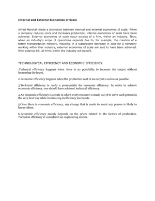
- 1. Internal and External Economies of Scale Alfred Marshall made a distinction between internal and external economies of scale. When a company reduces costs and increases production, internal economies of scale have been achieved. External economies of scale occur outside of a firm, within an industry. Thus, when an industry's scope of operations expands due to, for example, the creation of a better transportation network, resulting in a subsequent decrease in cost for a company working within that industry, external economies of scale are said to have been achieved. With external ES, all firms within the industry will benefit. TECHNOLOGYCAL EFFICIENCY AND ECONOMIC EFFICIENCY: .Technical efficiency happens when there is no possibility to increase the output without increasing the input. 2.Economic efficiency happens when the production cost of an output is as low as possible. 3.Technical efficiency is really a prerequisite for economic efficiency. In order to achieve economic efficiency, one should have achieved technical efficiency. 4.An economic efficiency is a state in which every resource is made use of to serve each person in the very best way while minimizing inefficiency and waste. 5.Once there is economic efficiency, any change that is made to assist any person is likely to harm others. 6.Economic efficiency mainly depends on the prices related to the factors of production. Technical efficiency is considered an engineering matter.
- 2. PRODUCTION FUNCTION: A function that specifies the output of a firm, an industry, or an entire economy for all combinations of inputs. this function is an assumed technological relationship, based on the current state of engineering knowledge; it does not represent the result of economic choices, but rather is an externally given entity that influences economic decision-making. Long Run In the long run, firms change production levels in response to (expected) economic profits or losses, and the land, labor, capital goods and entrepreneurs vary to reach associated long-run average cost (Figure 1). In the simplified case of plant capacity as the only fixed factor, a generic firm can make these changes in the long run: enter an industry in response to (expected) profits leave an industry in response to losses increase its plant in response to profits decrease its plant in response to losses. The long run is a planning and implementation stage. Here a firm may decide that it needs to produce on a larger scale by building a new plant or adding a production line. The firm may decide that new technology should be incorporated into its production process. The firm thus considers all its long-run production options and selects the optimal combination of inputs and technology for its long-run purposes. The optimal combination of inputs is the least-cost combination of inputs for desired level of output when all inputs are variable. Once the decisions are made and implemented and production begins, the firm is operating in the short run with fixed and variable inputs. Short Run All production in real time occurs in the short run. The short run is the conceptual time period in which at least one factor of production is fixed in amount and others are variable in amount. Costs that are fixed, say from existing plant size, have no impact on a firm's short-run decisions, since only variable costs and revenues affect short-run profits. Such fixed costs raise the associated short-run average cost of an output long-run average cost if the amount of the fixed factor is better suited for a different output level. In the short run, a firm can raise output by increasing the amount of the variable factor(s), such as labor through overtime. A generic firm already producing in an industry can make three changes in the short run as a response to reach a posited equilibrium: increase production decrease production shut down. The law of variable proportions states that as the quantity of one factor is increased, keeping the other factors fixed, the marginal product of that factor will eventually decline. This means that upto the use of a certain amount of variable factor, marginal product of the factor may increase and after a certain stage it starts diminishing. When the variable factor becomes relatively abundant, the marginal product may become negative. Assumptions: The law of variable proportions holds good under the following conditions: 1. 2. Constant State of Technology: First, the state of technology is assumed to be given and unchanged. If there is improvement in the technology, then the marginal product may rise instead of diminishing. Fixed Amount of Other Factors: Secondly, there must be some inputs whose quantity is kept fixed. It is only in this way that we can alter the factor proportions and know its effects on output. The law does not apply if all factors are proportionately varied.
- 3. 3. Possibility of Varying the Factor proportions: Thirdly, the law is based upon the possibility of varying the proportions in which the various factors can be combined to produce a product. The law does not apply if the factors must be used in fixed proportions to yield a product. Illustration of the Law: The law of variable proportion is illustrated in the following table and figure. Suppose there is a given amount of land in which more and more labour (variable factor) is used to produce wheat. Units of Labour Total Product Marginal Product Average Product 1 2 2 2 2 6 4 3 3 12 6 4 4 16 4 4 5 18 2 3.6 6 18 0 3 7 14 -4 2 8 8 -6 1 It can be seen from the table that upto the use of 3 units of labour, total product increases at an increasing rate and beyond the third unit total product increases at a diminishing rate. This fact is shown by the marginal product which is the addition made to Total Product as a result of increasing the variable factor i.e. labour. It can be seen from the table that the marginal product of labour initially rises and beyond the use of three units of labour, it starts diminishing. The use of six units of labour does not add anything to the total production of wheat. Hence, the marginal product of labour has fallen to zero. Beyond the use of six units of labour, total product diminishes and therefore marginal product of labour becomes negative. Regarding the average product of labour, it rises up to the use of third unit of labour and beyond that it is falling throughout. Three Stages of the Law of Variable Proportions: These stages are illustrated in the following figure where labour is measured on the X-axis and output on the Y-axis. Stage 1. Stage of Increasing Returns: In this stage, total product increases at an increasing rate up to a point. This is because the efficiency of the fixed factors increases as additional units of the variable factors are added to it. In the figure, from the origin to the point F, slope of the total product curve TP is increasing i.e. the curve TP is concave upwards upto the point F, which means that the marginal product MP of labour rises. The point F where the total product stops increasing at an increasing rate and starts increasing at a diminishing rate is called the point of inflection. Corresponding vertically to this point of inflection marginal product of labour is maximum, after which it diminishes. This stage is called the stage of increasing returns because the average product of the variable factor increases throughout this stage. This stage ends at the point where the average product curve reaches its highest point.
- 4. Stage 2. Stage of Diminishing Returns: In this stage, total product continues to increase but at a diminishing rate until it reaches its maximum point H where the second stage ends. In this stage both the marginal product and average product of labour are diminishing but are positive. This is because the fixed factor becomes inadequate relative to the quantity of the variable factor. At the end of the second stage, i.e., at point M marginal product of labour is zero which corresponds to the maximum point H of the total product curve TP. This stage is important because the firm will seek to produce in this range. Stage 3. Stage of Negative Returns: In stage 3, total product declines and therefore the TP curve slopes downward. As a result, marginal product of labour is negative and the MP curve falls below the Xaxis. In this stage the variable factor (labour) is too much relative to the fixed factor. Importance and Applicability of the Law of Variable Proportion: The Law of Variable Proportion has universal applicability in any branch of production. It forms the basis of a number of doctrines in economics. The Malthusian theory of population stems from the fact that food supply does not increase faster than the growth in population because of the operation of the law of diminishing returns in agriculture. Ricardo also based his theory of rent on this principle. According to him rent arises because the operation of the law of diminishing return forces the application of additional doses of labour and capital on a piece of land. Similarly the law of diminishing marginal utility and that of diminishing marginal physical productivity in the theory of distribution are also based on this theory. The law is of fundamental importance for understanding the problems of underdeveloped countries. In such agricultural economies the pressure of population on land increases with the increase in population. This leads to declining or even zero or negative marginal productivity of workers. This explains the operation of the law of diminishing returns in LDCs in its intensive form. Ragnar Nurkse have suggested ways to make use of these disguisedly unemployed labour by withdrawing them and putting them in those occupations where the marginal productivity is positive.