

Recomendados
Mais conteúdo relacionado
Mais procurados
Mais procurados (20)
Semelhante a Form 4 formulae and note
Semelhante a Form 4 formulae and note (20)
Mais de smktsj2
Mais de smktsj2 (20)
Form 4 formulae and note
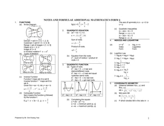
- 1. NOTES AND FORMULAE ADDITIONAL MATHEMATICS FORM 4 1. FUNCTIONS 2 6 The axis of symmetry is x – p = 0 or (a) Arrow Diagram fg(x) = f( )= 2 x=p x x (c) Quadratic inequalities 2. QUADRATIC EQUATION (x – a)(x – b) 0 2 (a) ax + bx + c = 0 Range x a, x b 2 x = b b 4ac (x – a)(x – b) 0 2a Range a x b Sum of roots: 4. INDICES AND LOGARITHM Domain = set A = {−2, 1, 2, 3} b Codomain = set B = {1, 4, 8, 9} n Range = set of images = {1, 4, 9} a (a) x=a loga x = n Object of 4 = −2, 2 Product of roots: Index Logarithm Image of 3 = 9 c Form Form 2 In function notation f : x x a (b) Types of Relation (b) Logrithm Law (b) Equation from the roots: 1. logaxy = logax + logay 2 x - (sum of roots)x + product of 2. loga x = logax – logay roots = 0 y n One-to-one One-to-many 3. loga x = n logax 3. QUADRATIC FUNCTION 4. loga a = 1 (a) Types of roots 5. loga 1 = 0 2 b - 4ac > 0 2 real and 6. loga b = log c b distinct/different roots. Many-to-one Many-to-many 2 log c a b - 4ac = 0 2 real and equal roots/two same roots. 7. loga b = 1 (c) Inverse Function 2 b - 4ac < 0 no real root. log b a Function f maps set A to set B 2 -1 b - 4ac 0 got real roots. Inverse function f maps set B to y y y set A. 5. COORDINATE GEOMETRY Given f(x) = ax + b, let y = ax + b (a) Distance between A(x1, y1) and y b -1 xb B(x2, y2) x= f :x 0 x a a 0 AB = ( x 2 x1 ) 2 ( y 2 y1 ) 2 x (d) Composite Function 0 x (b) Mid point AB 2 2 2 fg(x) means the function g followed b - 4ac > 0 b - 4ac = 0 b - 4ac < 0 M x1 x 2 , y1 y 2 by the function f. 2 2 2 (b) Completing the square E.g. f : x 3x – 2, g : x 2 (c) P which divides AB in the ratio m : n x y = a(x - p) + q a +ve minimum point (p, q) a –ve maximum point(p, q) Prepared by Mr. Sim Kwang Yaw 1
- 2. m : n By Histogram : x fx Frequency P B(x2 , y2 ) f A(x 1 , y1 ) For ungrouped data with frequency. P nx1 mx 2 ny1 my 2 fx , x i nm nm f (d) Gradient AB For grouped data, xi = mid-point m = y 2 y1 x 2 x1 (b) Median The data in the centre when 0 Mode Class boundary m = y-intercept arranged in order (ascending or x-intercept descending). (e) Equation of straight line Measurement of Dispersion (a) Interquartile Range Formula Formula : (i) Given m and A(x1, y1) 1 nF 1 M=L+ 2 C Q1 = L 4 n F1 C y – y1 = m(x – x1) fm 1 f Q1 (ii) Given A(x1, y1) and L = Lower boundary of median 3 class. Q3 = L 4 n F3 C B(x2, y2) 3 f Q3 n = Total frequency y y1 y 2 y1 F = cumulative frequency before the x x1 x 2 x1 median class Ogive : fm = frequency of median class Cumulative frequency (a) Area of polygon C = class interval size L = 1 x1 x2 x3 ......... x1 By Ogive 3 __ 2 y1 y 2 y 3 y1 Cumulative Frequency 4 n (g) Parallel lines m1 = m2 n 1 __ n (h) Perpendicular lines 4 m1 m2 = -1. n __ 2 0 Q Q 3 Upper boundary 6. STATISTICS 1 Measurement of Central Tendency Interquartile range = Q3 – Q1 (a) Mean 0 Median Upper boundary (b) Variance, Standard Deviation x x n 2 (c) Mode Variance = (standard deviation) For ungrouped data Data with the highest frequency Prepared by Mr. Sim Kwang Yaw 2
- 3. 2 d (xn) = nxn-1 9. SOLUTIONS OF TRIANGLES ( x x) (c) (a) The Sine Rule n dx sin A sin B sin C d (axn) = anxn-1 , or, = x2 x 2 (d) a b c n dx a b c For ungrouped data (e) Differentiation of product sin A sin B sin C 2 d (uv) = u dv + v du The Ambiguous Case f ( x x) dx dx dx f 2 = fx x 2 (f) Differentiation of Quotient f d u v du u dv For grouped data dx 2 dx dx v v Two triangles of the same 7. CIRCULAR MEASURE (g) Differentiation of Composite measurements can be drawn given (b) Radian Degree Function C, AC and AB where AB < AC. 0 d (ax+b)n = n(ax+b)n-1 × a = 180 r dx (b) The Cosine Rue 2 2 2 a = b + c – 2bc cos A (c) Degree Radian (h) Stationary point dy = 0 b 2 c2 a 2 = rad cos A = o dx 180 Maximum point: 2bc (d) Length of arc dy = 0 and d 2 y < 0 s = r 10. INDEX NUMBER dx dx 2 (a) Price Index (e) Area of sector p1 2 Minimum point: I 100 A = 1 r = 1 rs 2 po 2 2 dy = 0 and d y > 0 p0 is the price in the base year. (f) Area of segment dx dx 2 2 A = 1 r ( – sin ) (b) Composite Index 2 (i) Rate of Change dy dy dx I IW 8. DIFFERENTIATION (a) Differentiation by First Principle dt dx dt W dy had y I = price index (j) Small changes: W = weightage dx x 0 x dy d (a) = 0 y . x (b) dx dx Prepared by Mr. Sim Kwang Yaw 3