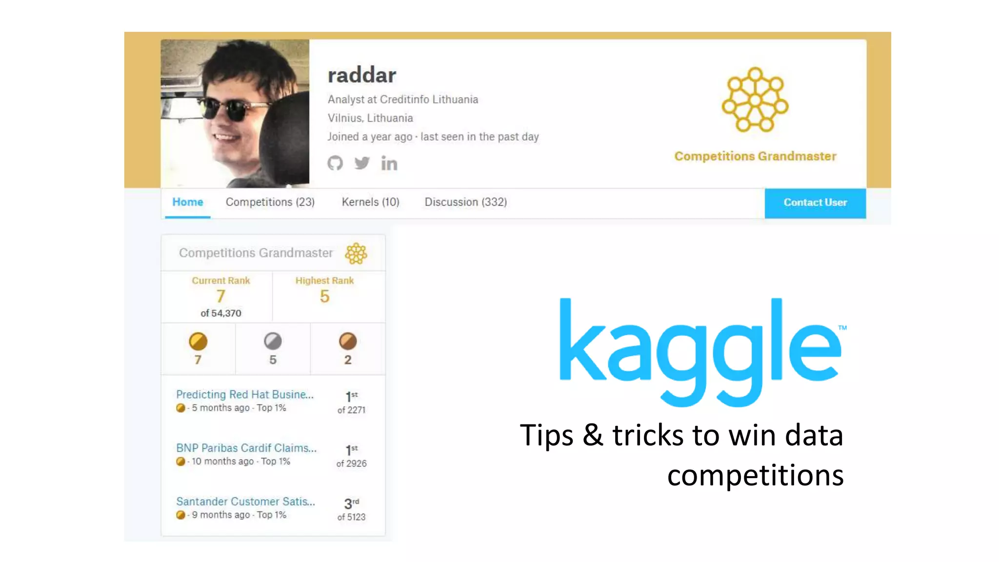
Tips and tricks to win kaggle data science competitions
The document serves as a guide for participating in predictive modeling competitions on platforms like Kaggle, emphasizing strategies for building competitive models and avoiding common pitfalls. It highlights the importance of cross-validation, feature engineering, and effective ensembling techniques while cautioning against overfitting and reliance on public leaderboard scores. Key tips include trusting cross-validation over public scores, using consistent CV splits, and the necessity of a robust data processing pipeline for improved model performance.
Overview of Kaggle as a platform for predictive modeling competitions, emphasizing collaboration, skills improvement, and competitive spirit.
Explanation of the predictive modeling workflow, including training and test sets, cross-validation, and model validation techniques.
Advice on avoiding overfitting to the public leaderboard scores and understanding their reliability.
Trust and reliability of cross-validation (CV) scores versus public leaderboard scores, highlighted by examples from competitions.
Introduction to bagging as a modeling approach, importance of reducing variance, and avoiding data leaks in training sets. Various encoding techniques for categorical features, emphasizing avoiding label leakage and optimizing model features.
Best practices for hyperparameter tuning and the significance of Bayesian optimization in parameter selection.
Tips for optimizing model performance with emphasis on feature engineering, model diversity, and the impact of ensembling.
Detailed exploration of ensembling methods such as voting, averaging, stacking, and tips for optimally selecting ensemble models.
Importance of feature engineering in model building, providing various transformation techniques and addressing data leakage.
Exploration of potential pitfalls in competition designs that may lead to data leakage and skewed results.
Final thoughts on competing in Kaggle, including the value of teamwork and forum discussions over individual solutions.
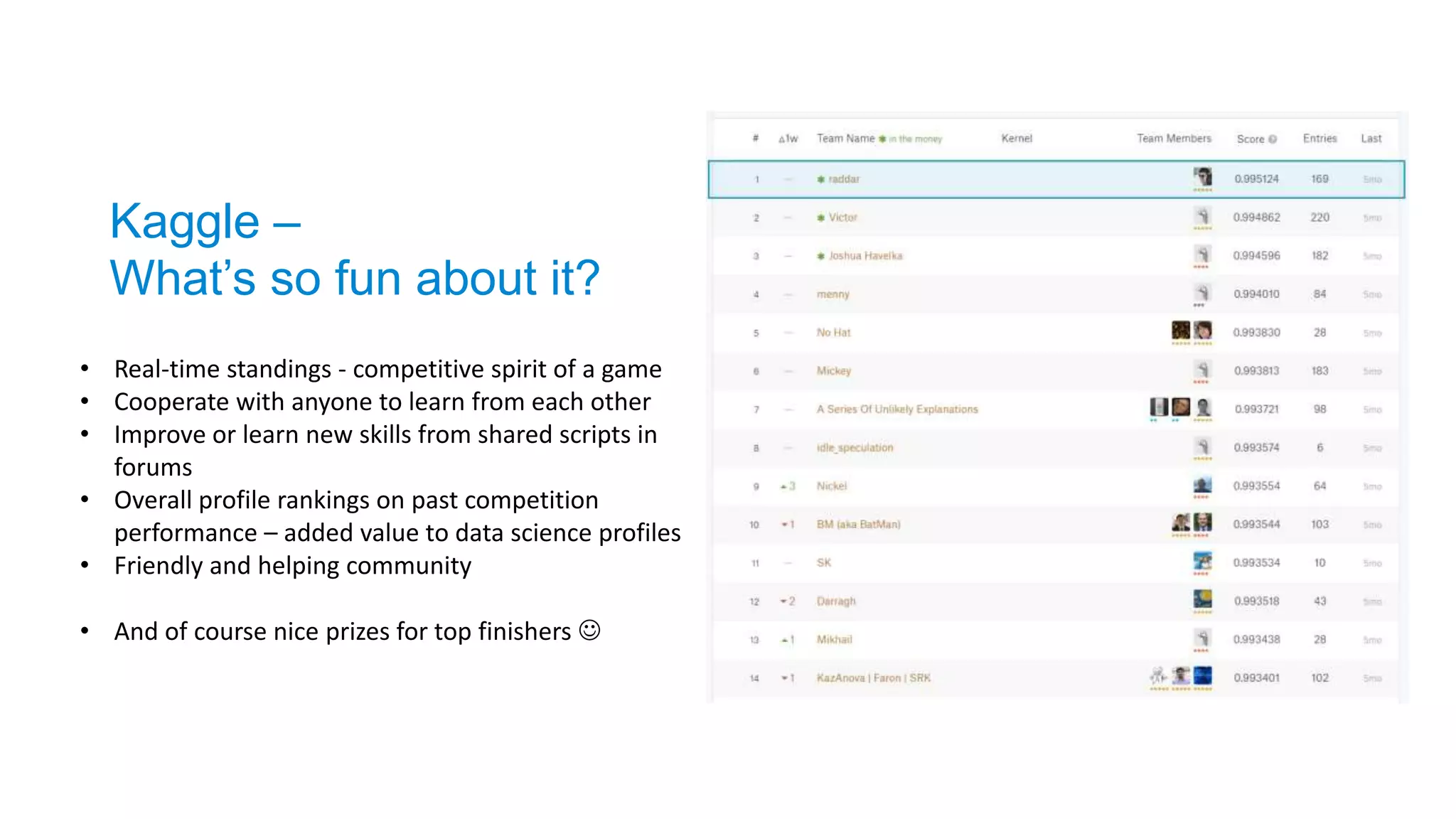
• Real-time standings- competitive spirit of a game
• Cooperate with anyone to learn from each other
• Improve or learn new skills from shared scripts in
forums
• Overall profile rankings on past competition
performance – added value to data science profiles
• Friendly and helping community
• And of course nice prizes for top finishers
Kaggle –
What’s so fun about it?
4.
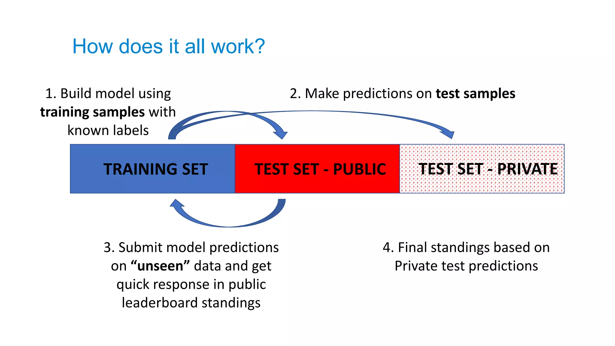
2. Make predictionson test samples1. Build model using
training samples with
known labels
TRAINING SET TEST SET - PUBLIC TEST SET - PRIVATE
3. Submit model predictions
on “unseen” data and get
quick response in public
leaderboard standings
4. Final standings based on
Private test predictions
How does it all work?
5.
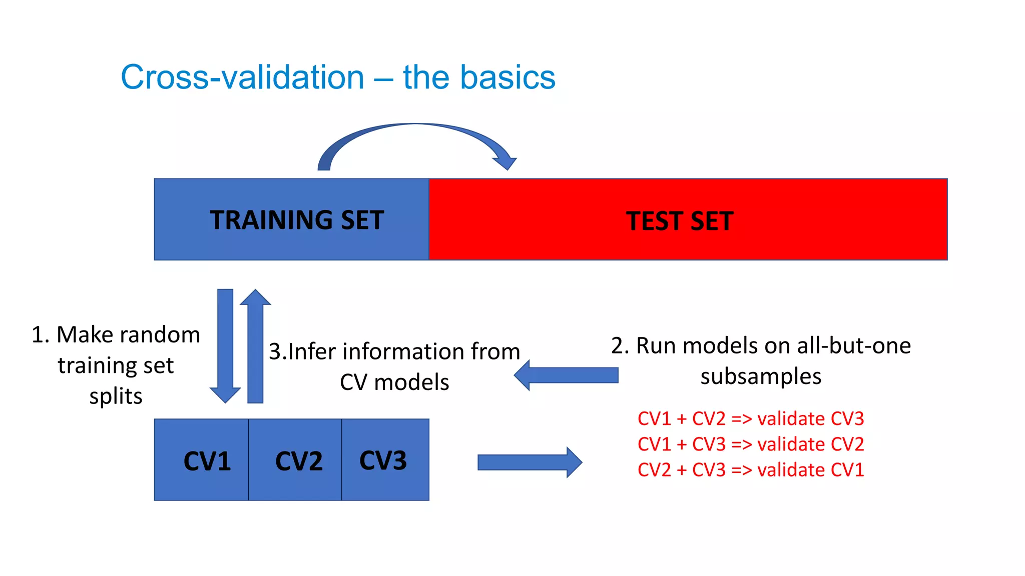
TRAINING SET TESTSET
1. Make random
training set
splits
3.Infer information from
CV models
CV1 CV2 CV3
CV1 + CV2 => validate CV3
CV1 + CV3 => validate CV2
CV2 + CV3 => validate CV1
2. Run models on all-but-one
subsamples
Cross-validation – the basics
6.
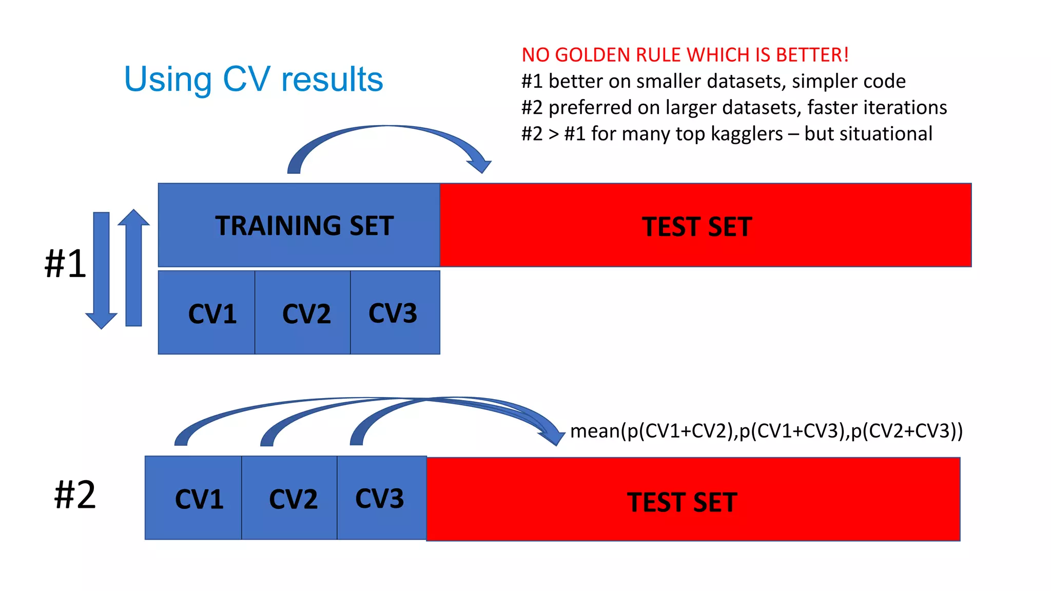
CV1 CV2 CV3TEST SET
CV1 CV2 CV3
mean(p(CV1+CV2),p(CV1+CV3),p(CV2+CV3))
NO GOLDEN RULE WHICH IS BETTER!
#1 better on smaller datasets, simpler code
#2 preferred on larger datasets, faster iterations
#2 > #1 for many top kagglers – but situational
#1
#2
TRAINING SET TEST SET
Using CV results
7.
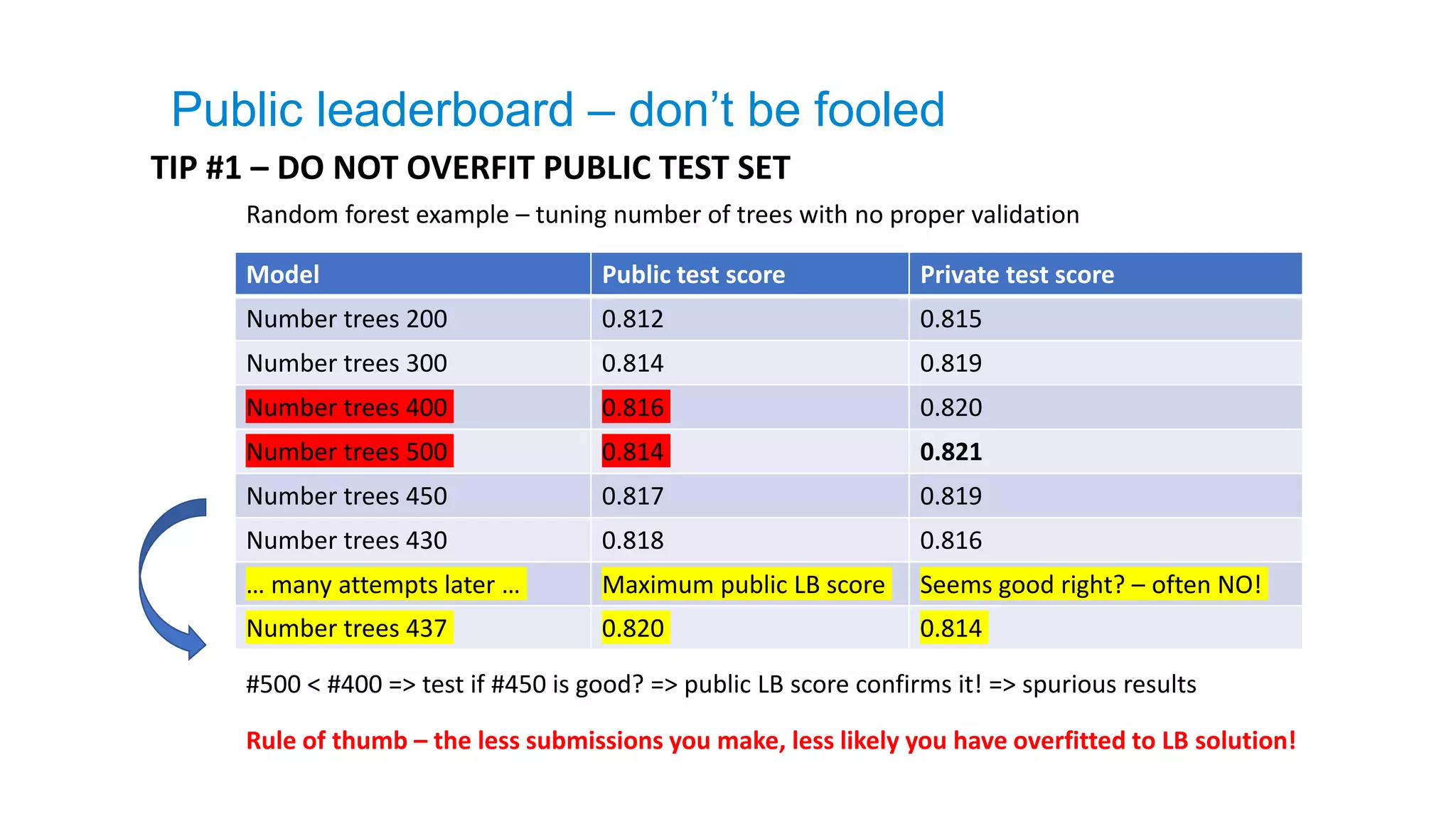
TIP #1 –DO NOT OVERFIT PUBLIC TEST SET
Model Public test score Private test score
Number trees 200 0.812 0.815
Number trees 300 0.814 0.819
Number trees 400 0.816 0.820
Number trees 500 0.814 0.821
Number trees 450 0.817 0.819
Number trees 430 0.818 0.816
… many attempts later … Maximum public LB score Seems good right? – often NO!
Number trees 437 0.820 0.814
Random forest example – tuning number of trees with no proper validation
#500 < #400 => test if #450 is good? => public LB score confirms it! => spurious results
Public leaderboard – don’t be fooled
Rule of thumb – the less submissions you make, less likely you have overfitted to LB solution!
8.
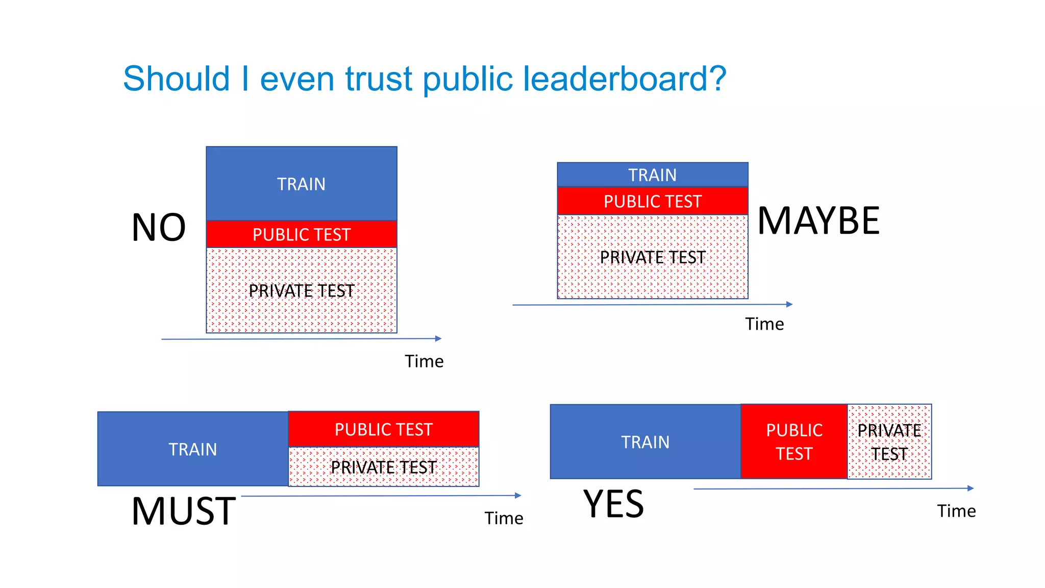
TRAIN
PUBLIC TEST
PRIVATE TEST
Time
TRAIN
PUBLICTEST
PRIVATE TEST
Time
NO MAYBE
TRAIN
PUBLIC TEST
PRIVATE TEST
TimeMUST
TRAIN
PUBLIC
TEST
PRIVATE
TEST
TimeYES
Should I even trust public leaderboard?
9.
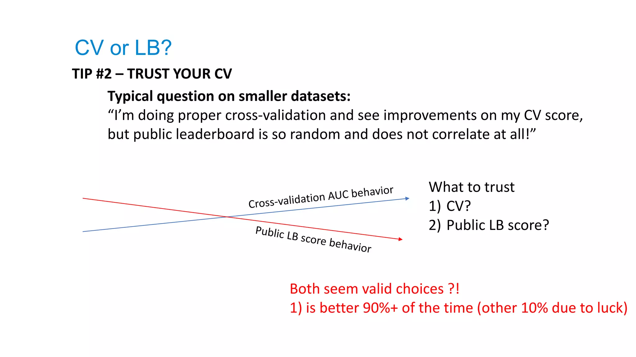
TIP #2 –TRUST YOUR CV
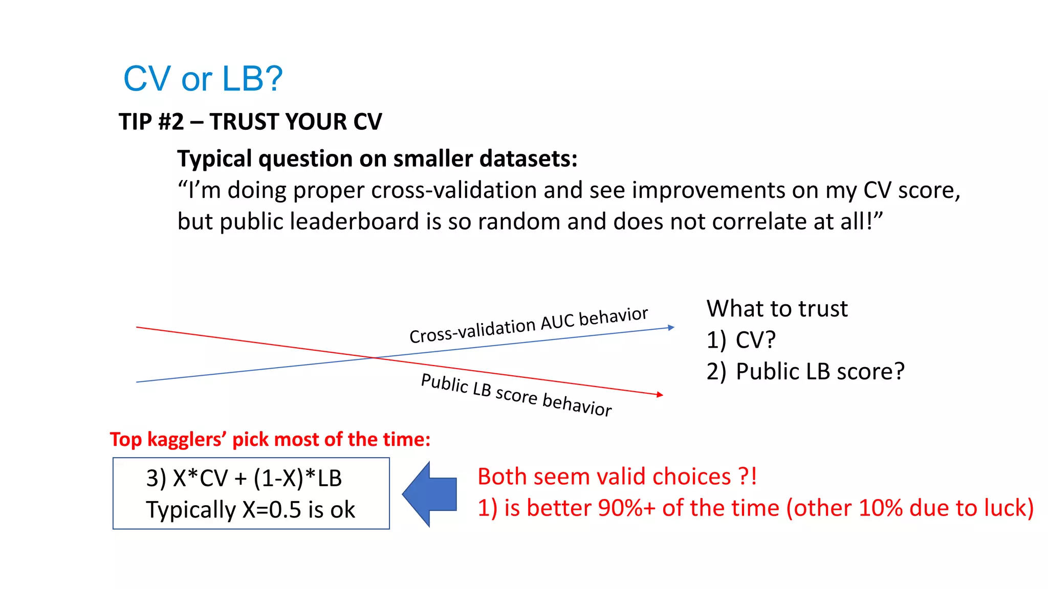
Typical question on smaller datasets:
“I’m doing proper cross-validation and see improvements on my CV score,
but public leaderboard is so random and does not correlate at all!”
What to trust
1) CV?
2) Public LB score?
Both seem valid choices ?!
1) is better 90%+ of the time (other 10% due to luck)
CV or LB?
10.
Typical question onsmaller datasets:
“I’m doing proper cross-validation and see improvements on my CV score,
but public leaderboard is so random and does not correlate at all!”
What to trust
1) CV?
2) Public LB score?
Both seem valid choices ?!
1) is better 90%+ of the time (other 10% due to luck)
3) X*CV + (1-X)*LB
Typically X=0.5 is ok
Top kagglers’ pick most of the time:
TIP #2 – TRUST YOUR CV
CV or LB?
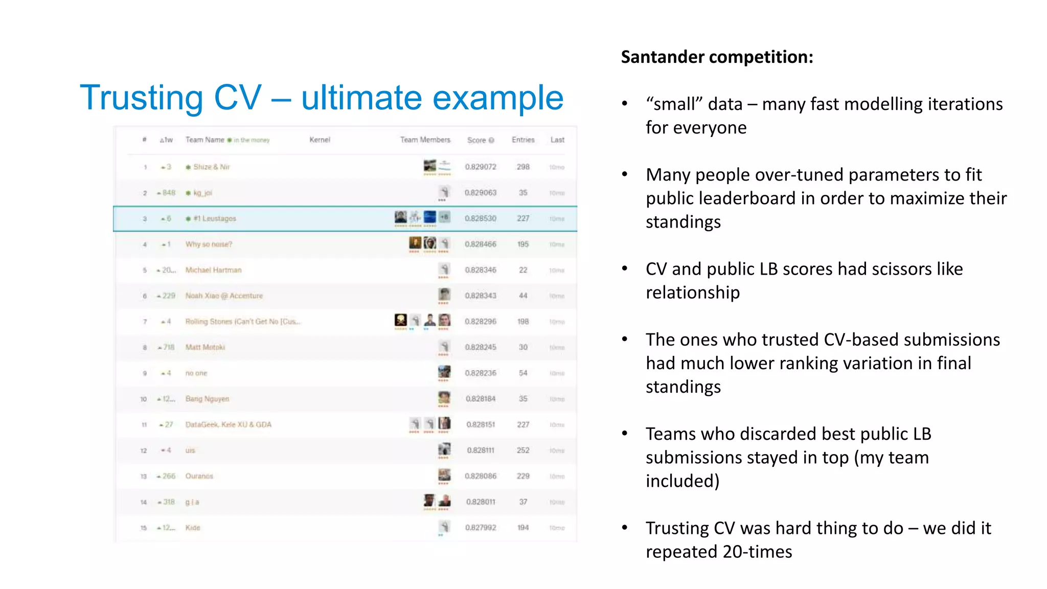
Santander competition:
• “small”data – many fast modelling iterations
for everyone
• Many people over-tuned parameters to fit
public leaderboard in order to maximize their
standings
• CV and public LB scores had scissors like
relationship
• The ones who trusted CV-based submissions
had much lower ranking variation in final
standings
• Teams who discarded best public LB
submissions stayed in top (my team
included)
• Trusting CV was hard thing to do – we did it
repeated 20-times
Trusting CV – ultimate example
13.
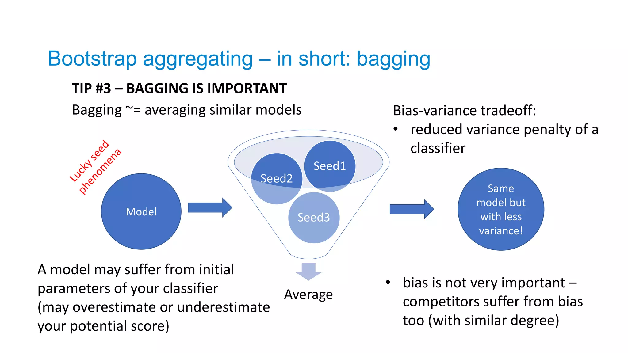
TIP #3 –BAGGING IS IMPORTANT
Average
Seed3
Seed2
Seed1
A model may suffer from initial
parameters of your classifier
(may overestimate or underestimate
your potential score)
Model
Same
model but
with less
variance!
Bagging ~= averaging similar models Bias-variance tradeoff:
• reduced variance penalty of a
classifier
• bias is not very important –
competitors suffer from bias
too (with similar degree)
Bootstrap aggregating – in short: bagging
14.
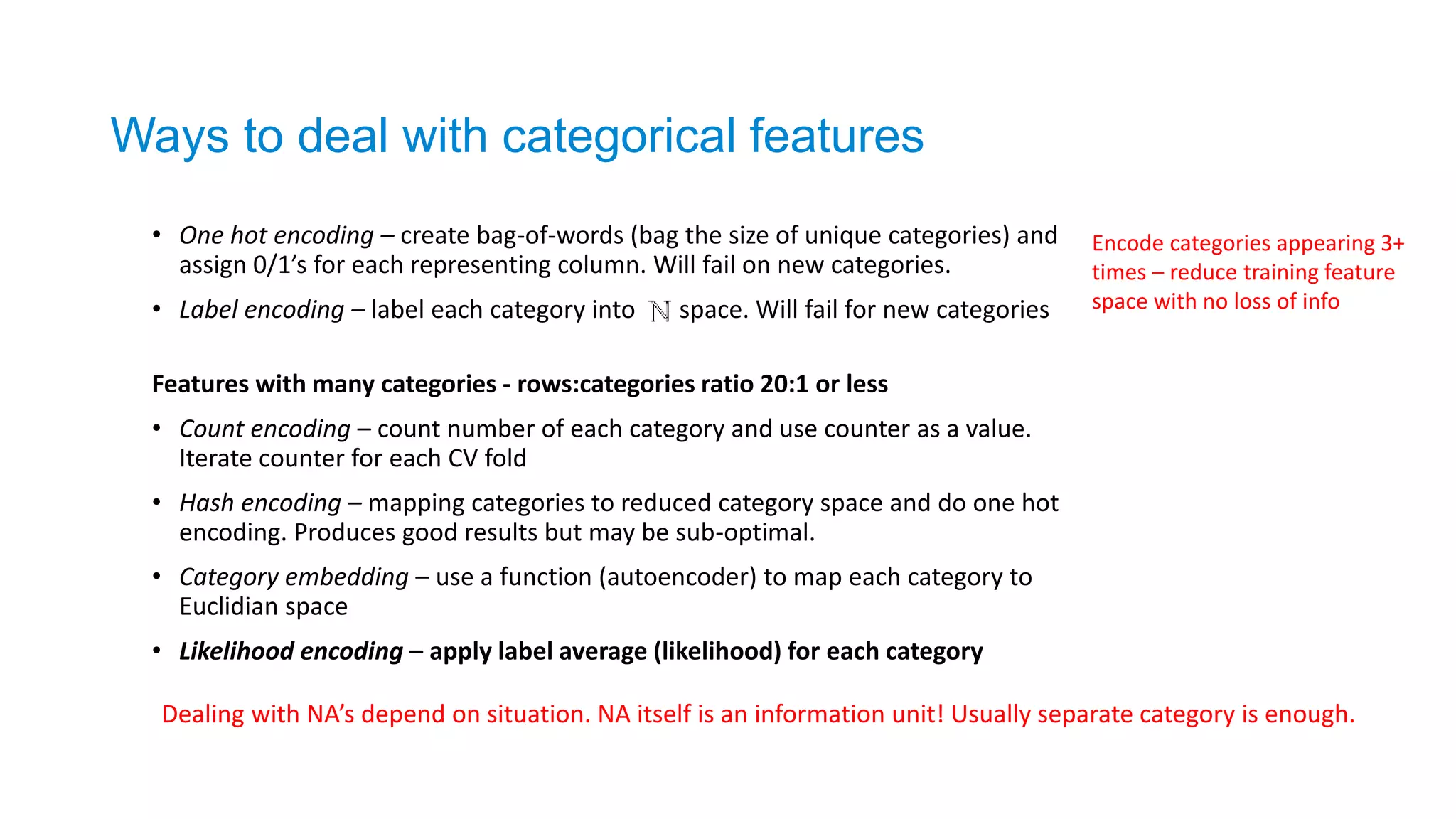
• One hotencoding – create bag-of-words (bag the size of unique categories) and
assign 0/1’s for each representing column. Will fail on new categories.
• Label encoding – label each category into space. Will fail for new categories
Features with many categories - rows:categories ratio 20:1 or less
• Count encoding – count number of each category and use counter as a value.
Iterate counter for each CV fold
• Hash encoding – mapping categories to reduced category space and do one hot
encoding. Produces good results but may be sub-optimal.
• Category embedding – use a function (autoencoder) to map each category to
Euclidian space
• Likelihood encoding – apply label average (likelihood) for each category
Ways to deal with categorical features
Encode categories appearing 3+
times – reduce training feature
space with no loss of info
Dealing with NA’s depend on situation. NA itself is an information unit! Usually separate category is enough.
15.
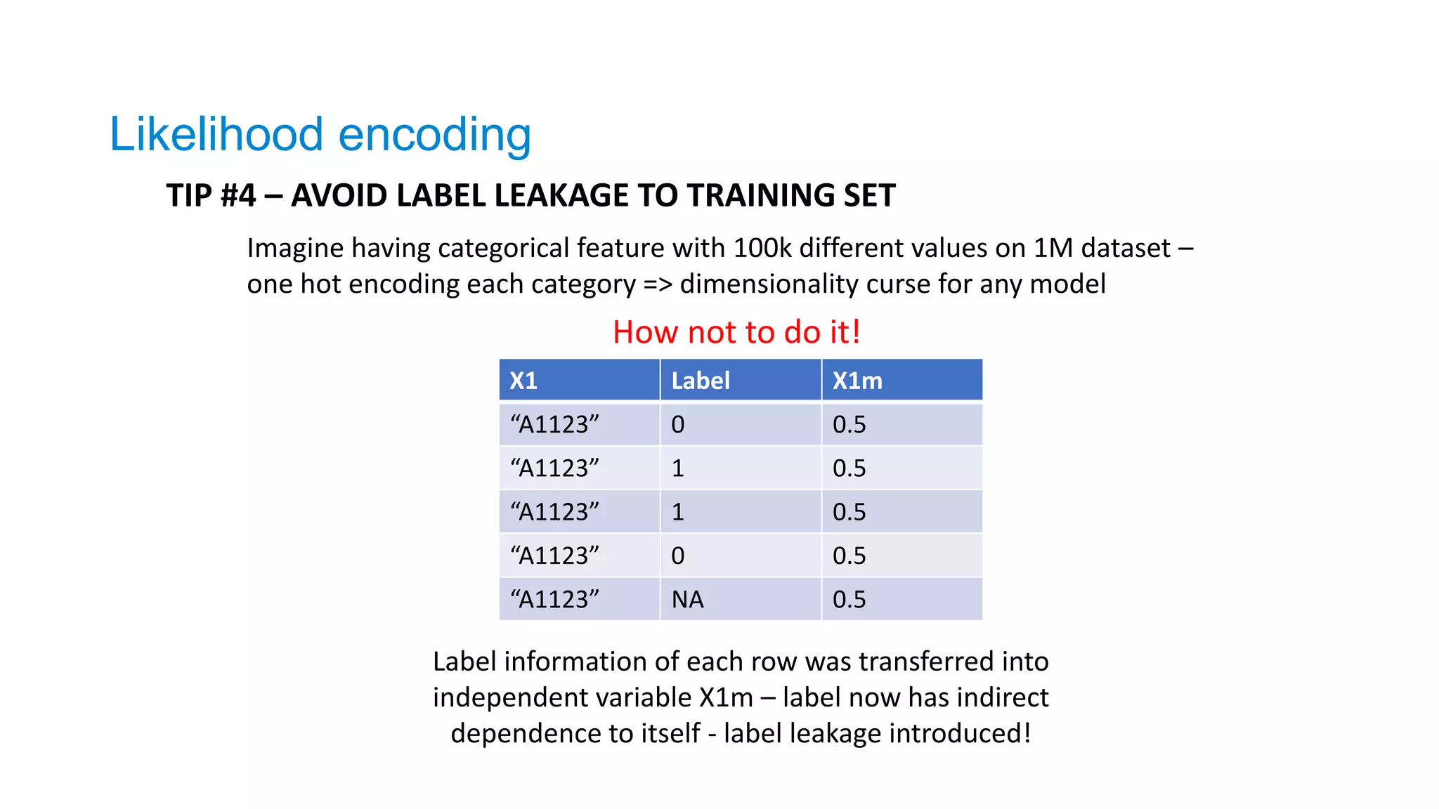
TIP #4 –AVOID LABEL LEAKAGE TO TRAINING SET
X1 Label X1m
“A1123” 0 0.5
“A1123” 1 0.5
“A1123” 1 0.5
“A1123” 0 0.5
“A1123” NA 0.5
How not to do it!
Label information of each row was transferred into
independent variable X1m – label now has indirect
dependence to itself - label leakage introduced!
Imagine having categorical feature with 100k different values on 1M dataset –
one hot encoding each category => dimensionality curse for any model
Likelihood encoding
16.
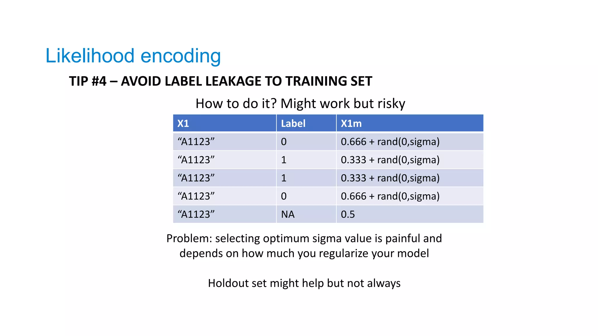
X1 Label X1m
“A1123”0 0.666 + rand(0,sigma)
“A1123” 1 0.333 + rand(0,sigma)
“A1123” 1 0.333 + rand(0,sigma)
“A1123” 0 0.666 + rand(0,sigma)
“A1123” NA 0.5
How to do it? Might work but risky
Problem: selecting optimum sigma value is painful and
depends on how much you regularize your model
Holdout set might help but not always
Likelihood encoding
TIP #4 – AVOID LABEL LEAKAGE TO TRAINING SET
17.
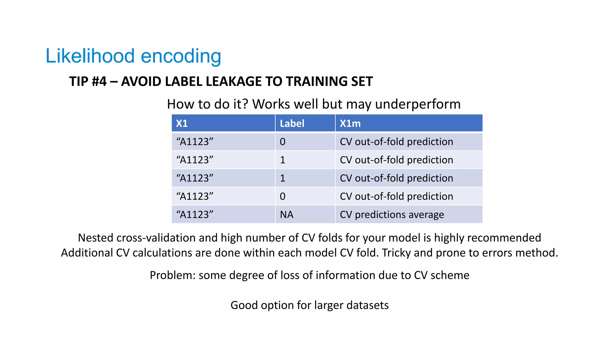
X1 Label X1m
“A1123”0 CV out-of-fold prediction
“A1123” 1 CV out-of-fold prediction
“A1123” 1 CV out-of-fold prediction
“A1123” 0 CV out-of-fold prediction
“A1123” NA CV predictions average
How to do it? Works well but may underperform
Nested cross-validation and high number of CV folds for your model is highly recommended
Additional CV calculations are done within each model CV fold. Tricky and prone to errors method.
Problem: some degree of loss of information due to CV scheme
Good option for larger datasets
Likelihood encoding
TIP #4 – AVOID LABEL LEAKAGE TO TRAINING SET
18.
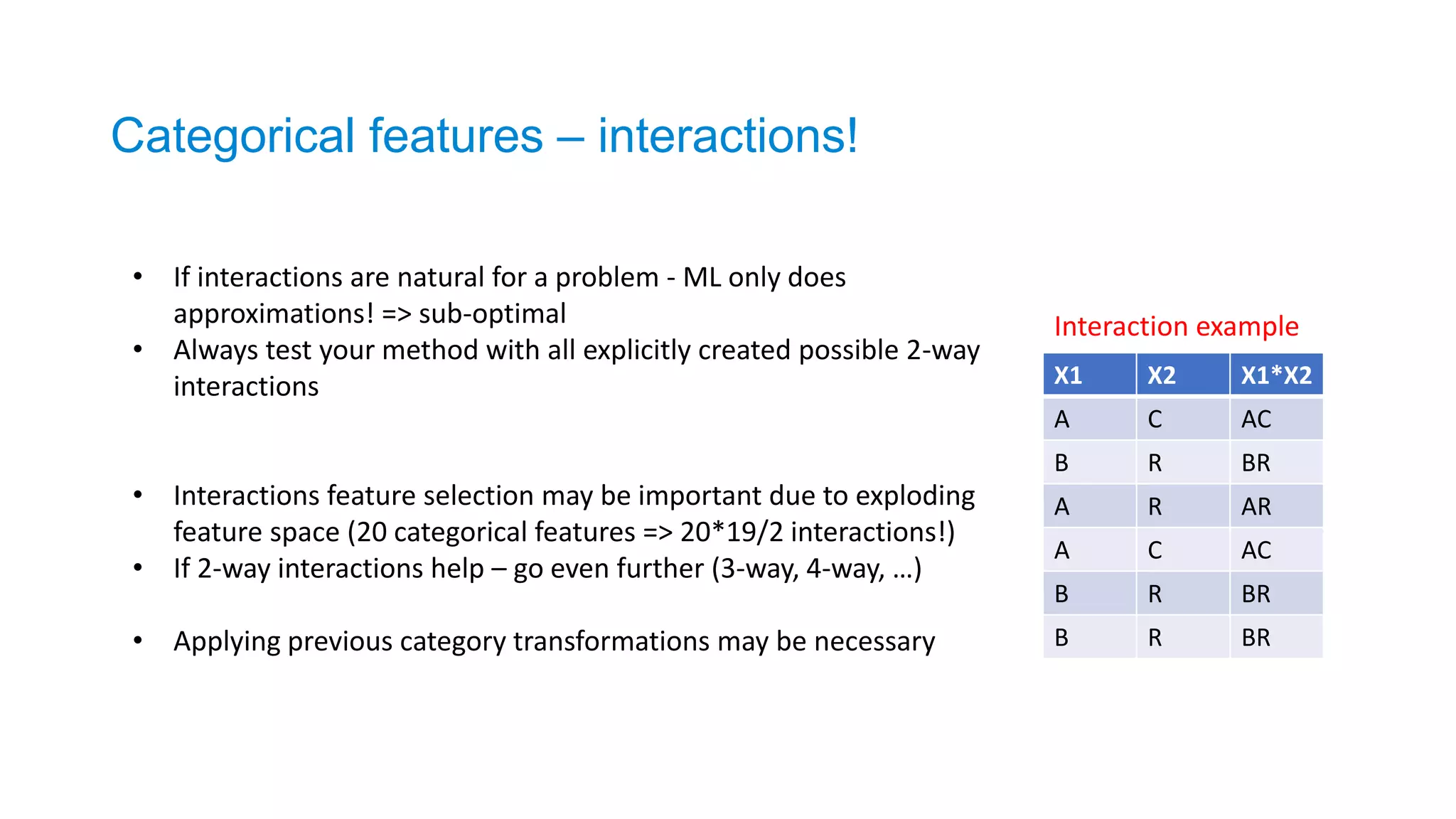
Categorical features –interactions!
• If interactions are natural for a problem - ML only does
approximations! => sub-optimal
• Always test your method with all explicitly created possible 2-way
interactions
• Interactions feature selection may be important due to exploding
feature space (20 categorical features => 20*19/2 interactions!)
• If 2-way interactions help – go even further (3-way, 4-way, …)
• Applying previous category transformations may be necessary
X1 X2 X1*X2
A C AC
B R BR
A R AR
A C AC
B R BR
B R BR
Interaction example
19.
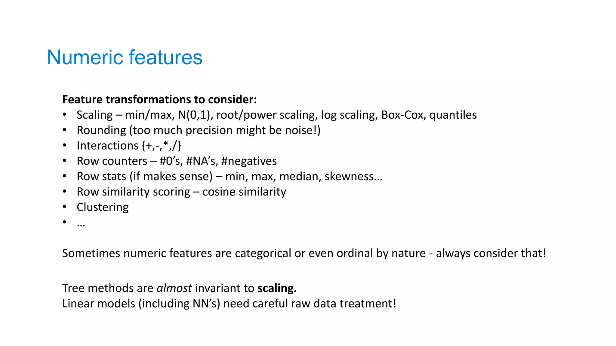
Numeric features
Feature transformationsto consider:
• Scaling – min/max, N(0,1), root/power scaling, log scaling, Box-Cox, quantiles
• Rounding (too much precision might be noise!)
• Interactions {+,-,*,/}
• Row counters – #0’s, #NA’s, #negatives
• Row stats (if makes sense) – min, max, median, skewness…
• Row similarity scoring – cosine similarity
• Clustering
• …
Sometimes numeric features are categorical or even ordinal by nature - always consider that!
Tree methods are almost invariant to scaling.
Linear models (including NN’s) need careful raw data treatment!
20.
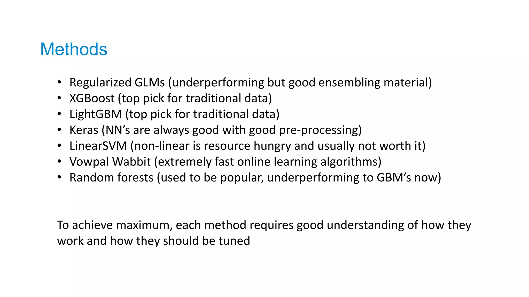
• Regularized GLMs(underperforming but good ensembling material)
• XGBoost (top pick for traditional data)
• LightGBM (top pick for traditional data)
• Keras (NN’s are always good with good pre-processing)
• LinearSVM (non-linear is resource hungry and usually not worth it)
• Vowpal Wabbit (extremely fast online learning algorithms)
• Random forests (used to be popular, underperforming to GBM’s now)
To achieve maximum, each method requires good understanding of how they
work and how they should be tuned
Methods
21.
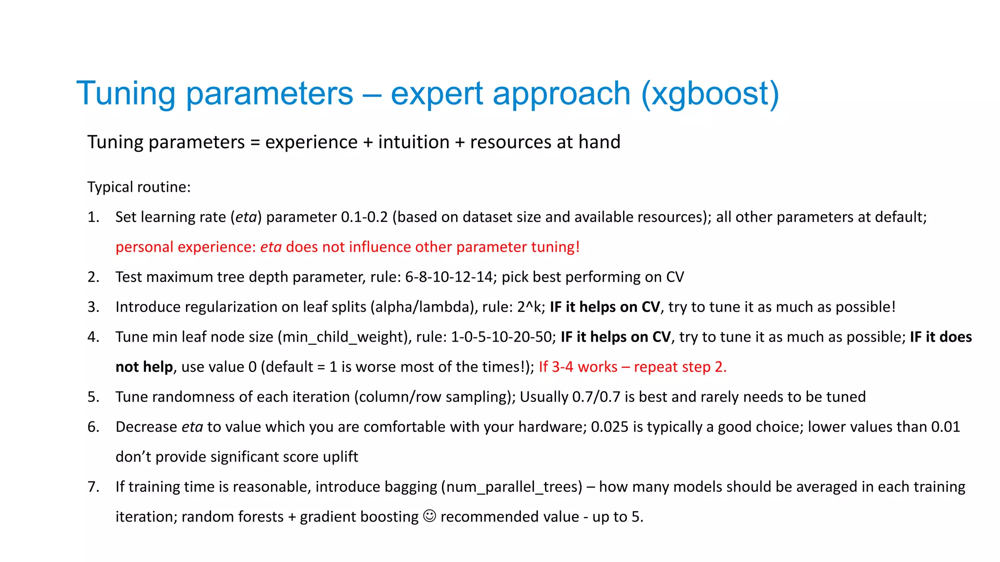
Tuning parameters =experience + intuition + resources at hand
Tuning parameters – expert approach (xgboost)
Typical routine:
1. Set learning rate (eta) parameter 0.1-0.2 (based on dataset size and available resources); all other parameters at default;
personal experience: eta does not influence other parameter tuning!
2. Test maximum tree depth parameter, rule: 6-8-10-12-14; pick best performing on CV
3. Introduce regularization on leaf splits (alpha/lambda), rule: 2^k; IF it helps on CV, try to tune it as much as possible!
4. Tune min leaf node size (min_child_weight), rule: 1-0-5-10-20-50; IF it helps on CV, try to tune it as much as possible; IF it does
not help, use value 0 (default = 1 is worse most of the times!); If 3-4 works – repeat step 2.
5. Tune randomness of each iteration (column/row sampling); Usually 0.7/0.7 is best and rarely needs to be tuned
6. Decrease eta to value which you are comfortable with your hardware; 0.025 is typically a good choice; lower values than 0.01
don’t provide significant score uplift
7. If training time is reasonable, introduce bagging (num_parallel_trees) – how many models should be averaged in each training
iteration; random forests + gradient boosting recommended value - up to 5.
22.
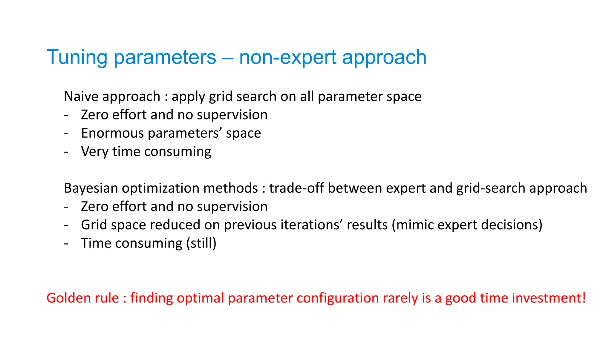
Naive approach :apply grid search on all parameter space
- Zero effort and no supervision
- Enormous parameters’ space
- Very time consuming
Bayesian optimization methods : trade-off between expert and grid-search approach
- Zero effort and no supervision
- Grid space reduced on previous iterations’ results (mimic expert decisions)
- Time consuming (still)
Tuning parameters – non-expert approach
Golden rule : finding optimal parameter configuration rarely is a good time investment!
23.
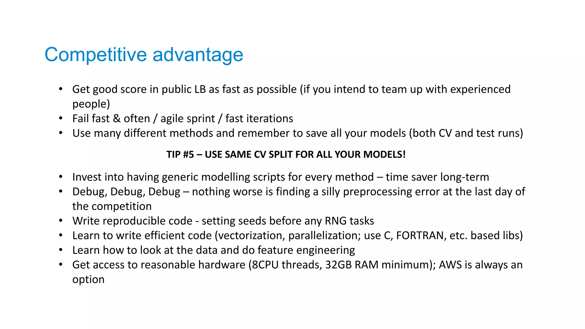
• Get goodscore in public LB as fast as possible (if you intend to team up with experienced
people)
• Fail fast & often / agile sprint / fast iterations
• Use many different methods and remember to save all your models (both CV and test runs)
• Invest into having generic modelling scripts for every method – time saver long-term
• Debug, Debug, Debug – nothing worse is finding a silly preprocessing error at the last day of
the competition
• Write reproducible code - setting seeds before any RNG tasks
• Learn to write efficient code (vectorization, parallelization; use C, FORTRAN, etc. based libs)
• Learn how to look at the data and do feature engineering
• Get access to reasonable hardware (8CPU threads, 32GB RAM minimum); AWS is always an
option
TIP #5 – USE SAME CV SPLIT FOR ALL YOUR MODELS!
Competitive advantage
24.
Ideally you wouldwant to have a framework which could be applied to any competition;
It should be:
• Data friendly (sparse/dense data, missing values, larger than memory)
• Problem friendly (classification, regression, clustering, ranking, etc.)
• Memory friendly (garbage collection, avoid using swap partition, etc.)
• Automated (runs unsupervised from data reading to generating submission files)
Competitive advantage – data flow pipeline
Good framework can save hours of repetitive work when going from one competition to another
25.
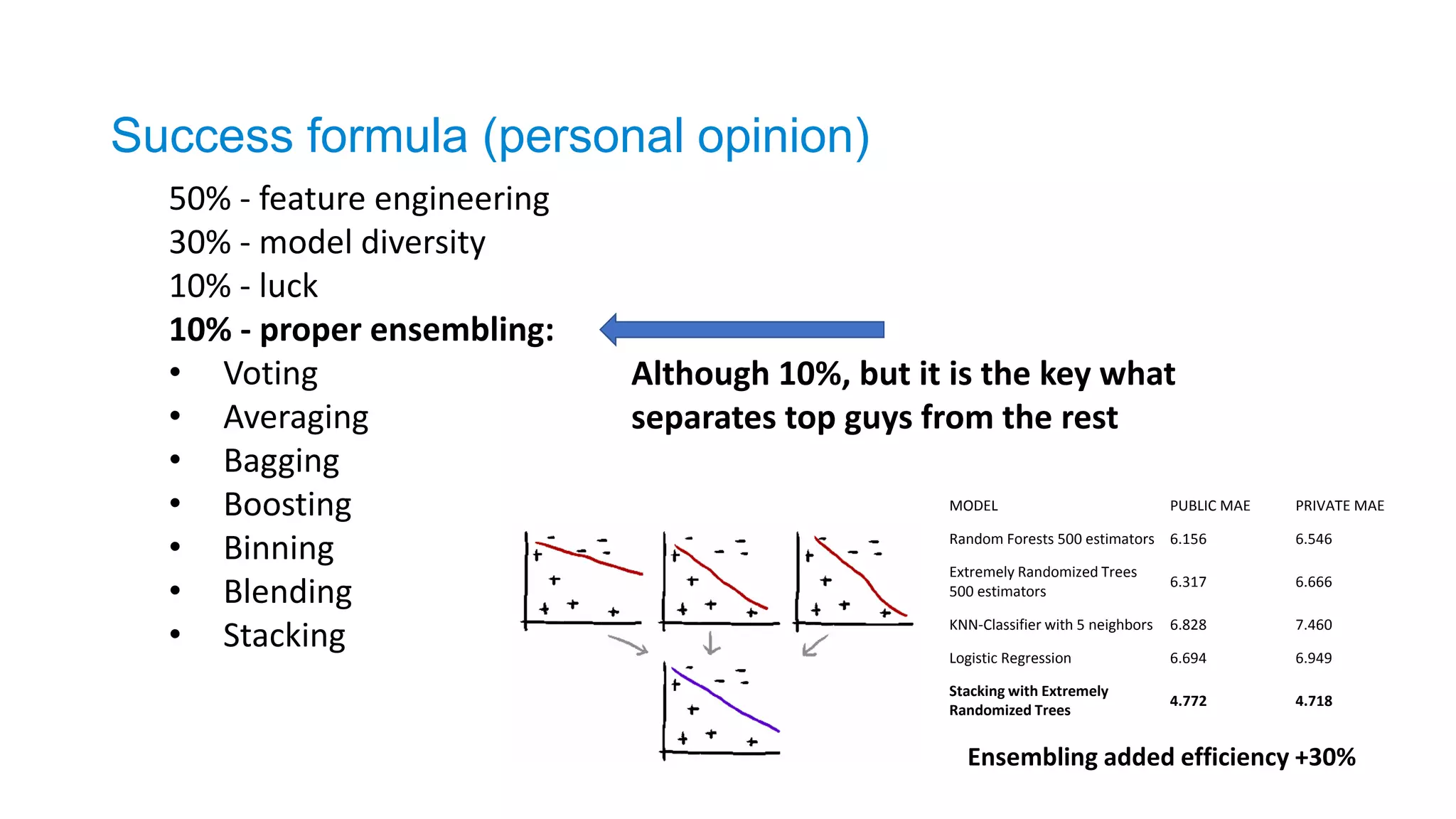
50% - featureengineering
30% - model diversity
10% - luck
10% - proper ensembling:
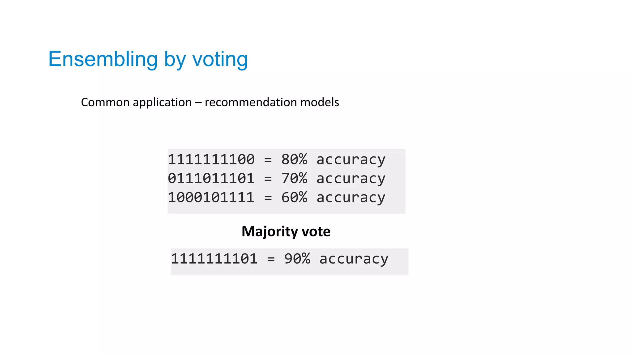
• Voting
• Averaging
• Bagging
• Boosting
• Binning
• Blending
• Stacking
Although 10%, but it is the key what
separates top guys from the rest
MODEL PUBLIC MAE PRIVATE MAE
Random Forests 500 estimators 6.156 6.546
Extremely Randomized Trees
500 estimators
6.317 6.666
KNN-Classifier with 5 neighbors 6.828 7.460
Logistic Regression 6.694 6.949
Stacking with Extremely
Randomized Trees
4.772 4.718
Ensembling added efficiency +30%
Success formula (personal opinion)
Ensembling by averaging
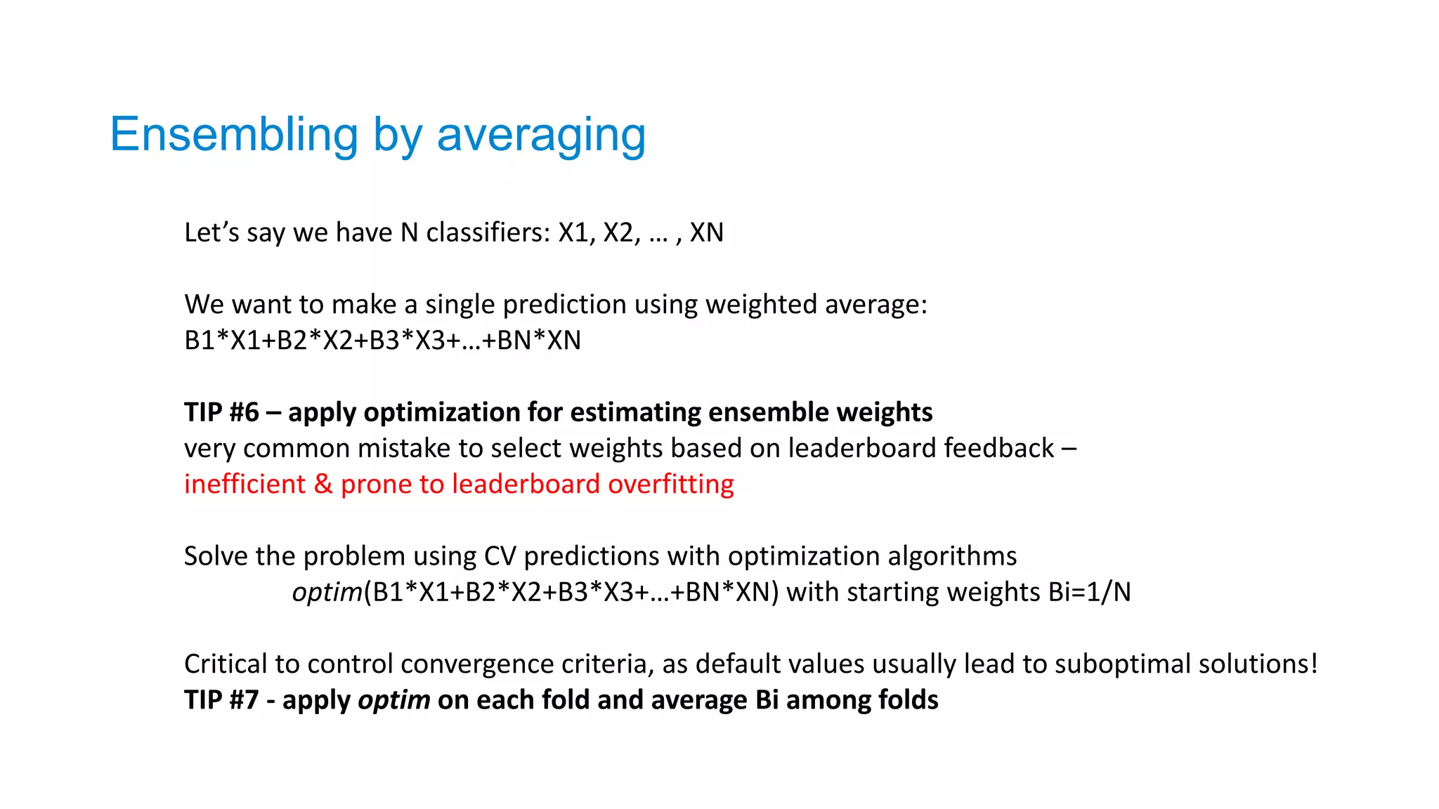
Let’ssay we have N classifiers: X1, X2, … , XN
We want to make a single prediction using weighted average:
B1*X1+B2*X2+B3*X3+…+BN*XN
TIP #6 – apply optimization for estimating ensemble weights
very common mistake to select weights based on leaderboard feedback –
inefficient & prone to leaderboard overfitting
Solve the problem using CV predictions with optimization algorithms
optim(B1*X1+B2*X2+B3*X3+…+BN*XN) with starting weights Bi=1/N
Critical to control convergence criteria, as default values usually lead to suboptimal solutions!
TIP #7 - apply optim on each fold and average Bi among folds
28.
Ensembling by averaging
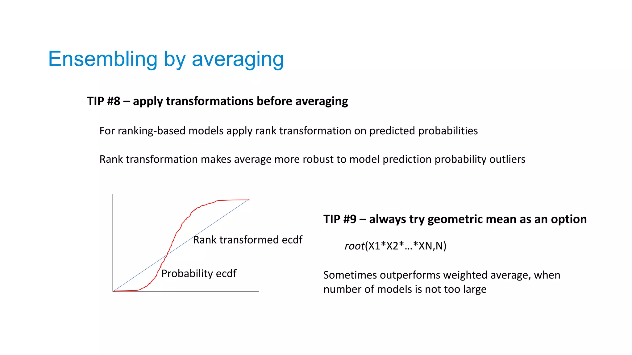
TIP#8 – apply transformations before averaging
For ranking-based models apply rank transformation on predicted probabilities
Rank transformation makes average more robust to model prediction probability outliers
Rank transformed ecdf
Probability ecdf
TIP #9 – always try geometric mean as an option
root(X1*X2*…*XN,N)
Sometimes outperforms weighted average, when
number of models is not too large
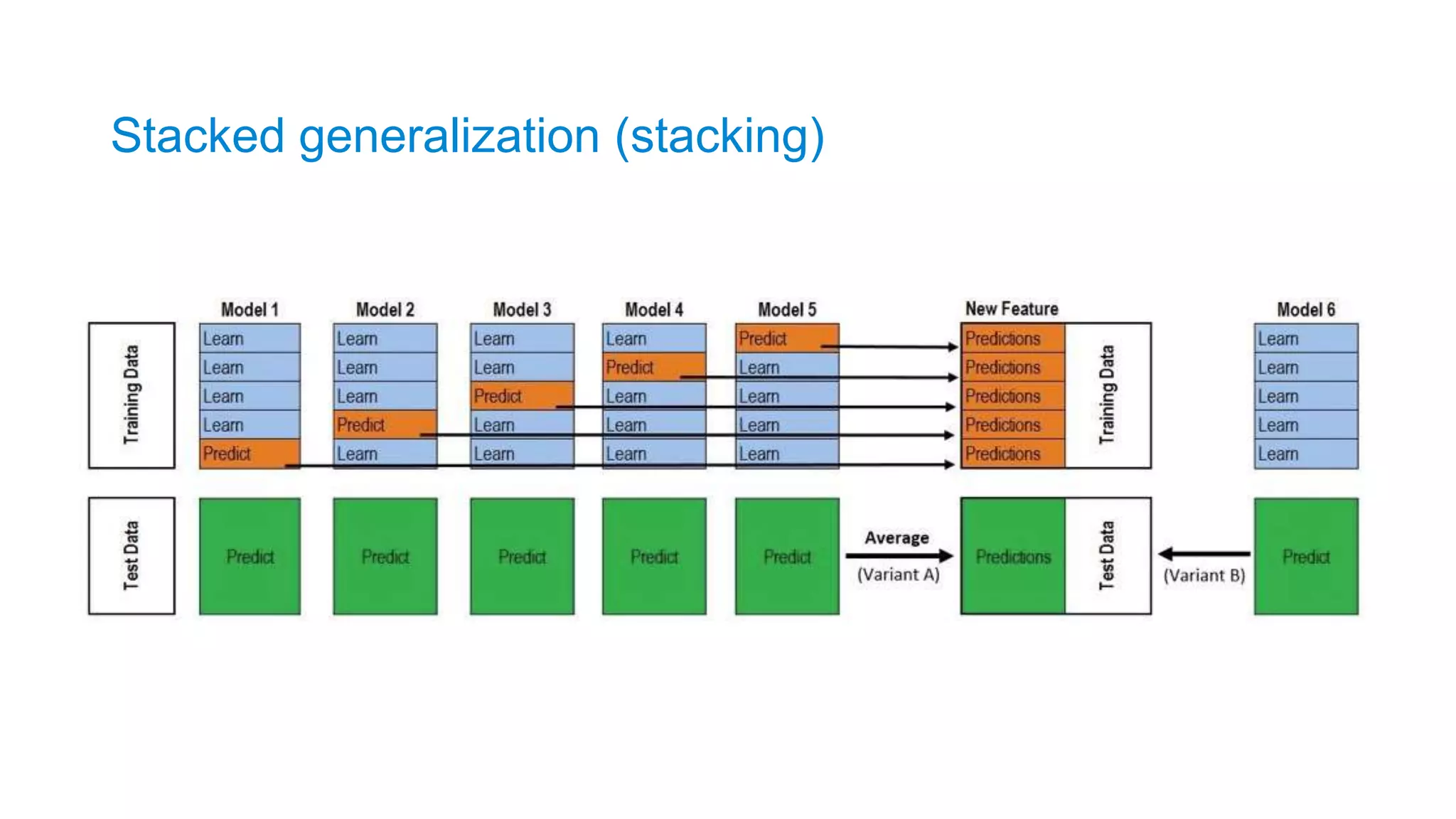
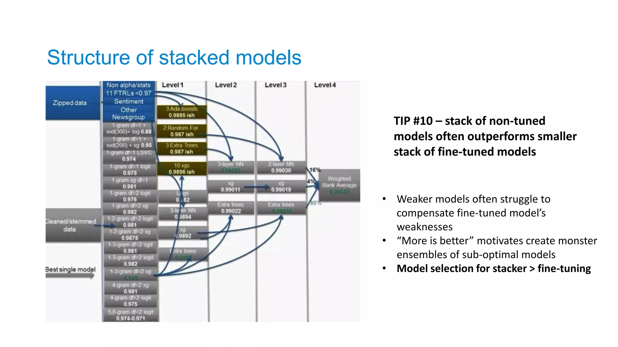
Structure of stackedmodels
TIP #10 – stack of non-tuned
models often outperforms smaller
stack of fine-tuned models
• Weaker models often struggle to
compensate fine-tuned model’s
weaknesses
• “More is better” motivates create monster
ensembles of sub-optimal models
• Model selection for stacker > fine-tuning
31.
Model selection forensemble
Having more models than necessary in ensemble may hurt.
Lets say we have a library of created models. Usually greedy-forward approach works well:
• Start with a few well-performing models’ ensemble
• Loop through each other model in a library and add to current ensemble
• Determine best performing ensemble configuration
• Repeat until metric converged
During each loop iteration it is wise to consider only a subset of library models, which could
work as a regularization for model selection.
Repeating procedure few times and bagging results reduces the possibility of overfitting by
doing model selection.
32.
0.4
0.41
0.42
0.43
0.44
0.45
0.46
Logloss
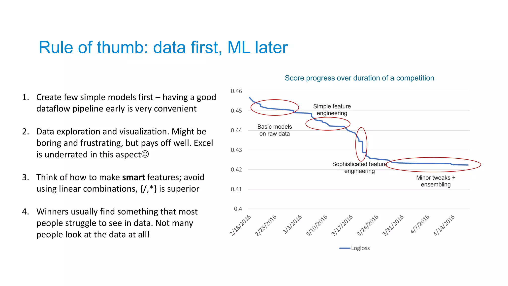
Score progress overduration of a competition
Basic models
on raw data
Simple feature
engineering
Sophisticated feature
engineering
Minor tweaks +
ensembling
Rule of thumb: data first, ML later
1. Create few simple models first – having a good
dataflow pipeline early is very convenient
2. Data exploration and visualization. Might be
boring and frustrating, but pays off well. Excel
is underrated in this aspect
3. Think of how to make smart features; avoid
using linear combinations, {/,*} is superior
4. Winners usually find something that most
people struggle to see in data. Not many
people look at the data at all!
Find something thatno one else can find = guaranteed top place finish
BNP Paribas competition:
• Medium sized dataset with 100+ anonymous features
• numerical features scaled to fit in [0; 20] interval, all looking like noise
• Dedicated 3 weeks for data exploration - found something no one else did
• Moving from i.i.d. dataset assumption to timetable dataset
• Whole new class of time related feature engineering
35.
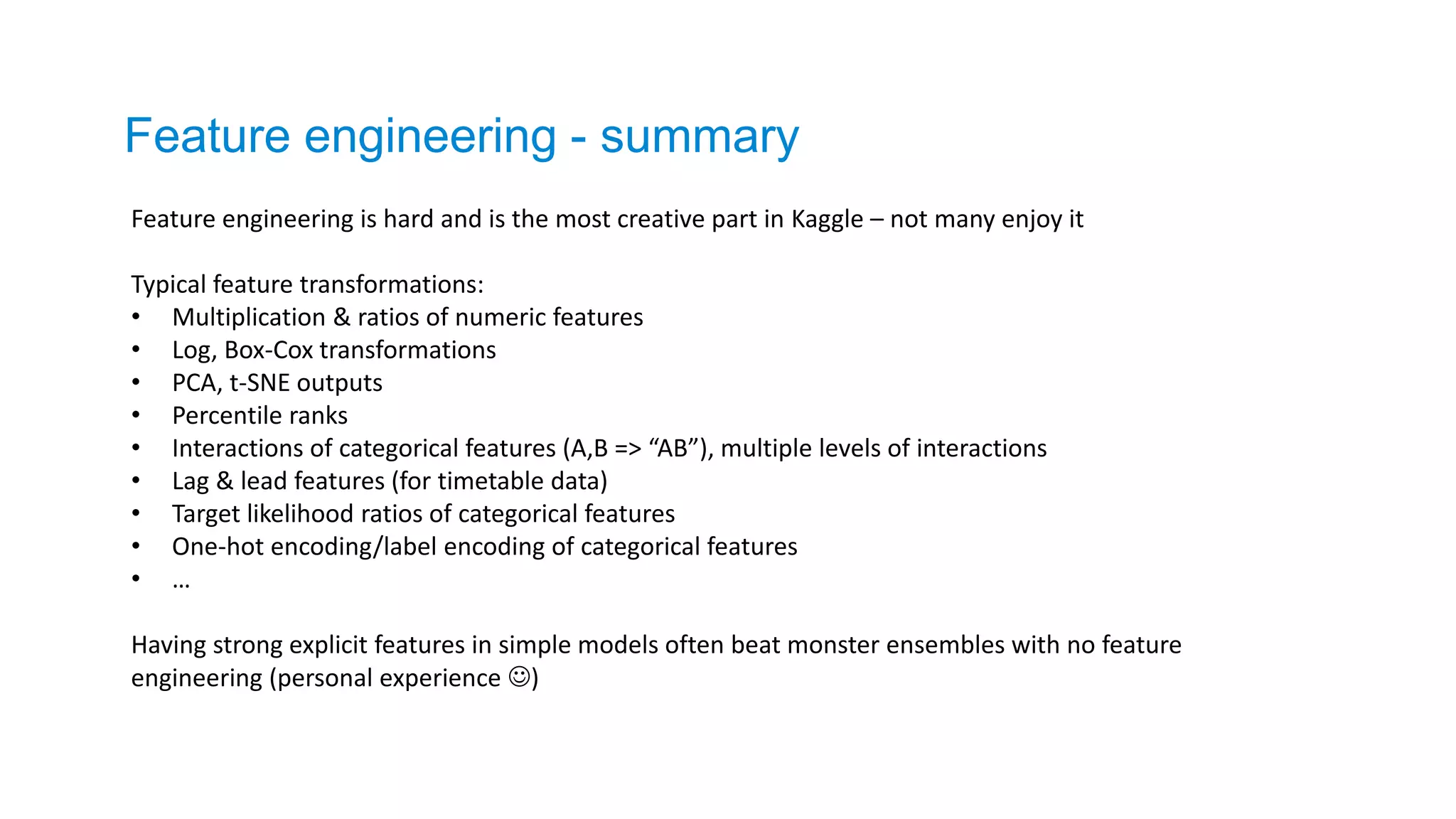
Feature engineering -summary
Feature engineering is hard and is the most creative part in Kaggle – not many enjoy it
Typical feature transformations:
• Multiplication & ratios of numeric features
• Log, Box-Cox transformations
• PCA, t-SNE outputs
• Percentile ranks
• Interactions of categorical features (A,B => “AB”), multiple levels of interactions
• Lag & lead features (for timetable data)
• Target likelihood ratios of categorical features
• One-hot encoding/label encoding of categorical features
• …
Having strong explicit features in simple models often beat monster ensembles with no feature
engineering (personal experience )
36.
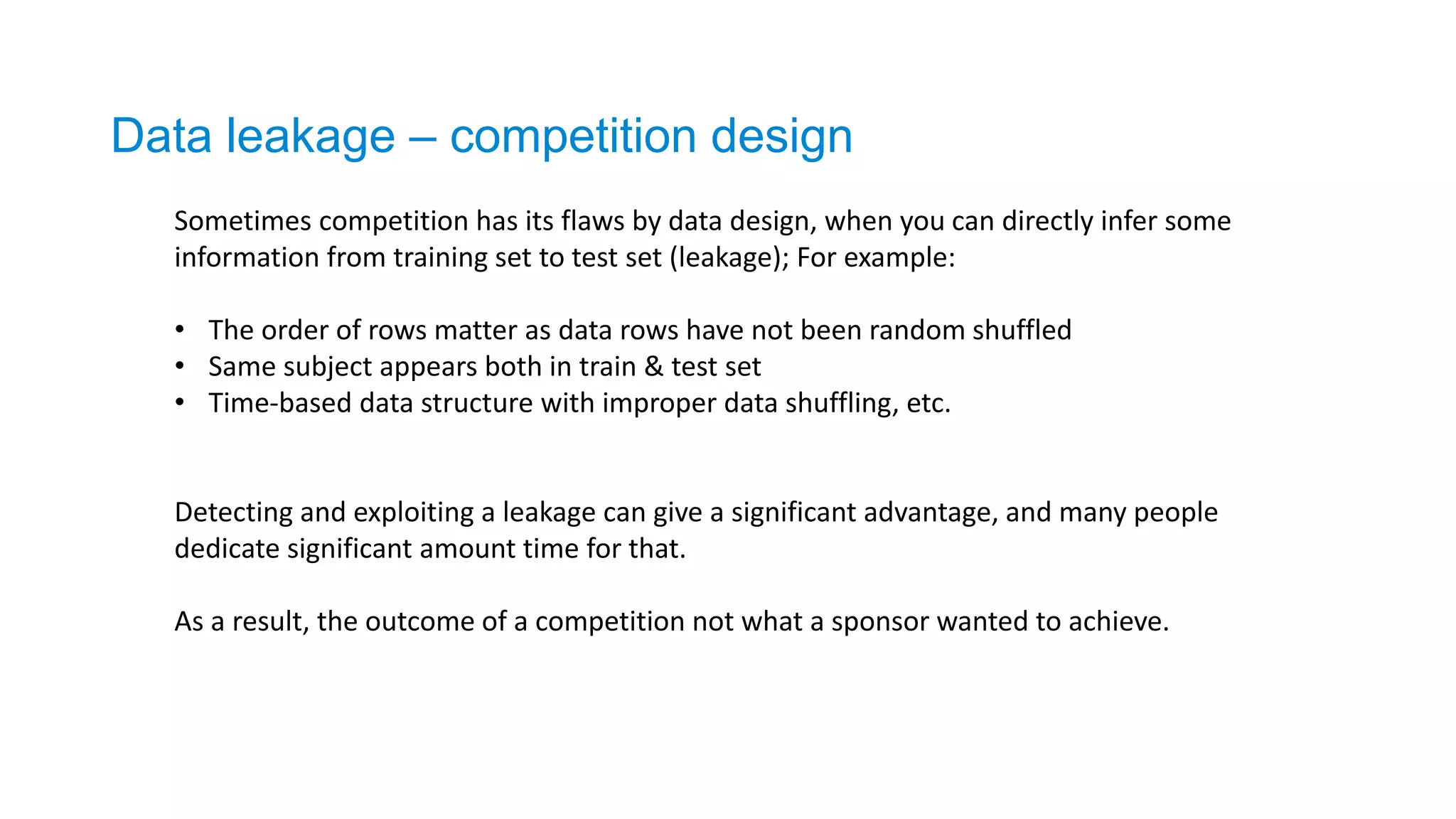
Data leakage –competition design
Sometimes competition has its flaws by data design, when you can directly infer some
information from training set to test set (leakage); For example:
• The order of rows matter as data rows have not been random shuffled
• Same subject appears both in train & test set
• Time-based data structure with improper data shuffling, etc.
Detecting and exploiting a leakage can give a significant advantage, and many people
dedicate significant amount time for that.
As a result, the outcome of a competition not what a sponsor wanted to achieve.
37.
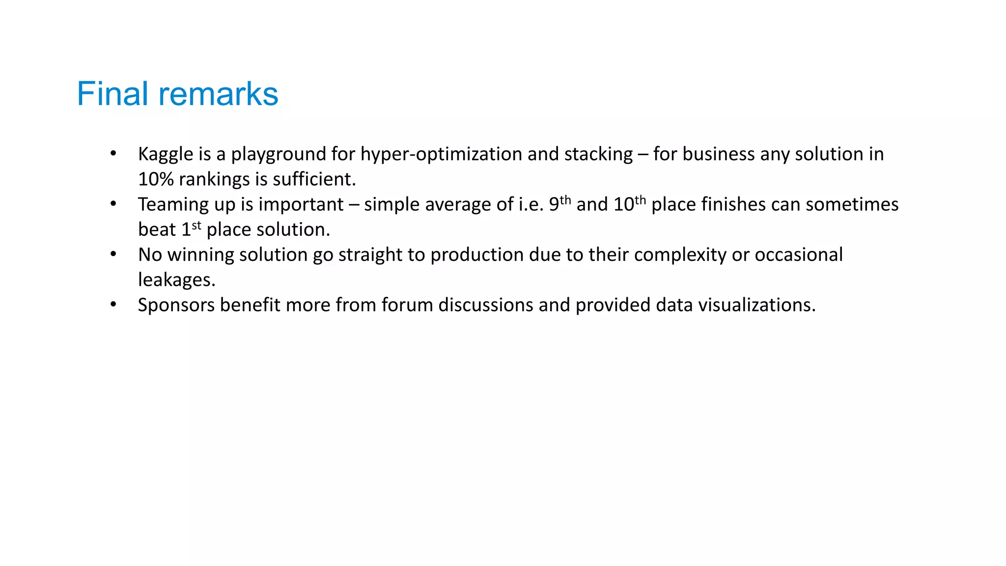
Final remarks
• Kaggleis a playground for hyper-optimization and stacking – for business any solution in
10% rankings is sufficient.
• Teaming up is important – simple average of i.e. 9th and 10th place finishes can sometimes
beat 1st place solution.
• No winning solution go straight to production due to their complexity or occasional
leakages.
• Sponsors benefit more from forum discussions and provided data visualizations.

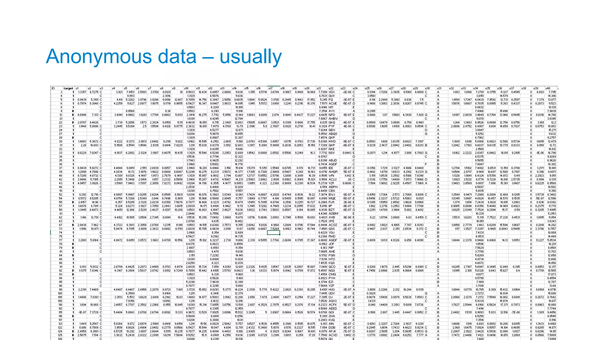
![Find something that no one else can find = guaranteed top place finish
BNP Paribas competition:
• Medium sized dataset with 100+ anonymous features
• numerical features scaled to fit in [0; 20] interval, all looking like noise
• Dedicated 3 weeks for data exploration - found something no one else did
• Moving from i.i.d. dataset assumption to timetable dataset
• Whole new class of time related feature engineering](https://image.slidesharecdn.com/kaggleraddarslides2017-02-06-170307165813/75/Tips-and-tricks-to-win-kaggle-data-science-competitions-34-2048.jpg)


![[ppt]](https://cdn.slidesharecdn.com/ss_thumbnails/ppt2931-thumbnail.jpg?width=640&height=640&fit=bounds)
![[ppt]](https://cdn.slidesharecdn.com/ss_thumbnails/ppt3441-thumbnail.jpg?width=640&height=640&fit=bounds)


