1. A&A 534, A37 (2011) Astronomy
DOI: 10.1051/0004-6361/201116870 &
c ESO 2011 Astrophysics
Multiwavelength campaign on Mrk 509
II. Analysis of high-quality Reflection Grating Spectrometer spectra
J. S. Kaastra1,2 , C. P. de Vries1 , K. C. Steenbrugge3,4 , R. G. Detmers1,2 , J. Ebrero1 , E. Behar5 , S. Bianchi6 ,
E. Costantini1 , G. A. Kriss7,8 , M. Mehdipour9 , S. Paltani10 , P.-O. Petrucci11 , C. Pinto1 , and G. Ponti12
1
SRON Netherlands Institute for Space Research, Sorbonnelaan 2, 3584 CA Utrecht, The Netherlands
e-mail: j.s.kaastra@stron.nl
2
Sterrenkundig Instituut, Universiteit Utrecht, PO Box 80000, 3508 TA Utrecht, The Netherlands
3
Instituto de Astronomía, Universidad Católica del Norte, Avenida Angamos 0610, Casilla 1280, Antofagasta, Chile
4
Department of Physics, University of Oxford, Keble Road, Oxford OX1 3RH, UK
5
Department of Physics, Technion-Israel Institute of Technology, Haifa 32000, Israel
6
Dipartimento di Fisica, Università degli Studi Roma Tre, via della Vasca Navale 84, 00146 Roma, Italy
7
Space Telescope Science Institute, 3700 San Martin Drive, Baltimore, MD 21218, USA
8
Department of Physics and Astronomy, The Johns Hopkins University, Baltimore, MD 21218, USA
9
Mullard Space Science Laboratory, University College London, Holmbury St. Mary, Dorking, Surrey, RH5 6NT, UK
10
ISDC Data Centre for Astrophysics, Astronomical Observatory of the University of Geneva, 16 ch. d’Ecogia, 1290 Versoix,
Switzerland
11
UJF-Grenoble 1 / CNRS-INSU, Institut de Planétologie et d’Astrophysique de Grenoble (IPAG), UMR 5274, Grenoble 38041,
France
12
School of Physics and Astronomy, University of Southampton, Highfield, Southampton SO17 1BJ, UK
Received 11 March 2011 / Accepted 11 July 2011
ABSTRACT
Aims. We study the bright Seyfert 1 galaxy Mrk 509 with the Reflection Grating Spectrometers (RGS) of XMM-Newton, using for
the first time the RGS multi-pointing mode of XMM-Newton to constrain the properties of the outflow in this object. We obtain very
accurate spectral properties from a 600 ks spectrogram of Mrk 509 with excellent quality.
Methods. We derive an accurate relative calibration for the effective area of the RGS and an accurate absolute wavelength calibration.
We improve the method for adding time-dependent spectra and enhance the efficiency of the spectral fitting by two orders of magni-
tude.
Results. Taking advantage of the spectral data quality when using the new RGS multi-pointing mode of XMM-Newton, we show that
the two velocity troughs previously observed in UV spectra are resolved.
Key words. galaxies: active – quasars: absorption lines – X-rays: general
1. Introduction with XMM-Newton spanning seven weeks in Oct.–Nov. 2009.
The properties of the outflow are derived from the high-
Outflows from active galactic nuclei (AGN) play an important resolution X-ray spectra taken with the Reflection Grating
role in the evolution of the super-massive black holes (SMBH) Spectrometers (RGS, den Herder et al. 2001) of XMM-Newton.
at the centres of the AGN, as well as on the evolution of the host The time-averaged RGS spectrum is one of the best spectra ever
galaxies and their surroundings. In order to better understand taken with this instrument, and the statistical quality of this spec-
the role of photo-ionised outflows, the geometry must be deter- trum can be used to improve the current accuracy of the cali-
mined. In particular, our goal is to determine the distance of the bration and analysis tools. This creates new challenges for the
photo-ionised gas to the SMBH, which currently has large un- analysis of the data. The methods developed here also apply to
certainties. For this reason we have started an extended monitor- other time-variable sources. Therefore we describe them in some
ing campaign on one of the brightest AGN with an outflow, the detail in this paper.
Seyfert 1 galaxy Mrk 509 (Kaastra et al. 2011). The main goal For this work we have derived a list of the strongest absorp-
of this campaign is to track the response of the photo-ionised gas tion lines in the X-ray spectrum of Mrk 509, and we perform
to the temporal variations of the ionising X-ray and UV contin- some simple line diagnostics on a few of the most prominent
uum. The response time immediately yields the recombination features. The full time-averaged spectrum will be presented else-
time scale and hence the density of the gas. Combining this with where (Detmers et al. 2011).
the ionisation parameter of the gas, the distance of the outflow
to the central SMBH can be determined.
The first step in this process is to accurately determine the 2. Data analysis
physical state of the outflow: what is the distribution of gas as
a function of ionisation parameter, how many velocity compo- Table 1 gives some details on our observations. We quote here
nents are present, how large is the turbulent line broadening, etc. only exposure times for RGS. The total net exposure time is
Our campaign on Mrk 509 is centred around ten observations 608 ks. No filtering for enhanced background radiation was
Article published by EDP Sciences A37, page 1 of 16
2. A&A 534, A37 (2011)
Table 1. Observation log. spectrum 1 + spectrum 2 = total spectrum residuals
800
texp = 1 s texp = 1 s texp = 2 s
Obs. ID Start date Net exposure
Nr. (ks) A B
600
1 0601390201 2009-10-15 60
"absorption"
2 0601390301 2009-10-19 53
"emission"
3 0601390401 2009-10-23 61 A B
4 0601390501 2009-10-29 60 400
Counts
5 0601390601 2009-11-02 63
6 0601390701 2009-11-06 63 A B
7 0601390801 2009-11-10 61 200 A B
8 0601390901 2009-11-14 60
9 0601391001 2009-11-18 65
10 0601391101 2009-11-20 63
0
needed for these observations, because the background was very
−200
low and stable for the full duration of our campaign.
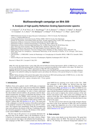
The campaign consisted of ten different observations. Each Fig. 1. Illustration that spectra with different flux and different miss-
observation was pointed a bit differently to obtain slightly differ- ing bins cannot be simply added. Both spectrum 1 and 2 have 1 s
ent positions of the spectra on the detectors (the multi-pointing exposure but have different constant expected count rates of 400 and
mode of RGS; steps of 0, ±15 and ±30 ). In this way the holes 200 counts s−1 . In spectrum 1 pixel A is missing, in spectrum 2 pixel B.
in the detector caused by bad CCD columns and pixels and CCD The thick solid line in the total spectrum indicates the predicted number
of counts by straightforwardly adding the response matrices for both
gaps, changed position over the spectra, allowing all spectral spectra with equal weights.
bins to be sampled. In addition, eventually this procedure will
limit outliers in individual wavelength bins from isolated noisy
CCD pixels, because the noise of these pixels will be spread over
more wavelength bins. pointings are combined, or if bad columns have (dis)appeared
between different observations because of the transient nature of
After all exposures were separately processed using the stan-
some bad pixels.
dard RGS pipeline of the XMM-Newton data analysis system
SAS version 9, noise from remaining noisy CCD columns and Under the above conditions the SAS task rgscombine should
pixels was decreased even more using the following process. not be used. We illustrate this with a simplified example (Fig. 1).
Two-dimensional plots of the spectral image (cross-dispersion Consider two spectra of the same X-ray source, labelled 1 and 2,
position versus dispersion angle) and the CCD-pulse height ver- with seven spectral bins each (Fig. 1). The source has a flat
sus spectral dispersion were plotted in the detector reference spectrum and the flux per bin in spectrum 1 is twice the flux
frame for each separate CCD node, but with all exposures com- of spectrum 2. In spectrum 1, bin A is missing (zero counts),
bined. Because the spectral features will be smeared out in these and in spectrum 2, bin B is missing. The combined spectrum has
plots, possible CCD defects like hot or dead columns and hot or 600 counts, except for bins A and B with 200 and 400 counts,
dead pixels are clearly visible. In this way a number of additional respectively. However, when the response matrices of both ob-
bad columns and pixels were manually identified for each detec- servations are combined, it is assumed that bins A and B were
tor CCD node and were added to the SAS bad pixel calibration on for 50% of the time, hence the model predicts 300 counts for
file. After this, all exposures were reprocessed with the new bad those bins. Clearly, the data show a deficit or excess at those bins,
pixel tables. which an observer could easily misinterpret as an additional as-
trophysical absorption or emission feature at bins A and B.
How can this problem be solved? One possibility is to fit
3. Combination of spectra all spectra simultaneously. However, when there are many dif-
ferent spectra (like the 40 spectra obtained from two RGS de-
To obtain an accurate relative effective area and absolute wave- tectors in two spectral orders for ten observations that we have
length calibration, we need the signal-to-noise of the combined for our Mrk 509 data), this can be a cumbersome procedure be-
600 ks spectrum. Therefore we first describe how the individual cause the memory and CPU requirements become very demand-
spectra are accurately combined, and discuss the effective area ing. Another option is to rigorously discard all wavelength bins
and wavelength scale later. where even during short periods (a single observation or a part of
an observation) data are lacking. This solution will cause a sig-
nificant loss of diagnostic capability, because many more bins
3.1. Combination of spectra from the same RGS
are discarded and likely several of those bins will be close to
and spectral order
astrophysically interesting features.
Detectors like the RGS yield spectra with lacking counts in Here we follow a different route. It is common wisdom (and
parts of the spectrum owing to the presence of hot pixels, bad this is also suggested by the SAS manual) not to use fluxed
columns, or gaps between CCDs. This leads to problems when spectra for fitting analyses. The problem is the lack of a well-
spectra taken at different times have to be combined into a single defined redistribution function for that case. We will show be-
spectrum, in particular when the source varies in intensity and low in Sect. 4 that we can obtain an appropriate response matrix
the lacking counts fall on different wavelengths for each indi- for our case, which allows us to make an analysis with fluxed
vidual spectrum. For RGS this is for example the case when the spectra under the conditions given in that section.
multi-pointing mode is used like in our present Mrk 509 cam- We first create individual fluxed spectra using the SAS task
paign, or when data of different epochs with slightly different rgsfluxer. We use exactly the same wavelength grid for each
A37, page 2 of 16
3. J. S. Kaastra et al.: Multiwavelength campaign on Mrk 509. II.
observation. We then average the fluxed spectra using for each
spectral bin the exposure times as weights. This is repeated for f = 1.0
all bins having 100% exposure and for all spectra that are to
combined.
For bins with lacking data (like bins A and B of Fig. 1) we
f = 0.5
have to follow a different approach. If the total exposure time of
spectrum k is given by tk , and the effective exposure time of spec-
Flux
tral bin j in spectrum k is given by tk j , we clearly have tk j < tk
for “problematic” bins j, and we will include in the final spec- f = 0.0
trum only data bins with tk j > f tk , with 0 ≤ f ≤ 1 a tunable
parameter discussed below. However, because of the variability
of the source, the average flux level of the included spectra k for
problematic bin j may differ from the flux level of the neigh-
bouring bins j − 1 and j + 1 which are fully exposed. To correct
for this, we assume that the spectral shape (but not the overall
normalisation) in the local neighbourhood of bin j is constant in 16 16.2 16.4 16.6 16.8 17
time. From these neighbouring bins (with fluxes F j−1 and F j+1 ) Wavelength (Å)
we estimate the relative contribution R to the total flux for the Fig. 2. Spectral region near the gap between CCD 5 and 6 of RGS2,
spectra k that have sufficient exposure time tk j for bin j, i.e. containing the 1s–3p line of O viii at 16.55 Å from the outflow. From
top to bottom we show the fluxed spectra (arbitrarily scaled and shifted
tk F j−1 along the flux axis) for three values of f . Using the conservative setting
k, tk j > f tk
R≡ , (1) f = 1, a major part of the spectrum is lost. With f = 0 no data are lost
tk F j−1 but of course between 16.3 and 16.55 Å the error bars are slightly larger
k because of the shorter exposure time in that wavelength region.
and similar for the other neighbour at j + 1. We interpolate the
values for R linearly at both sides to obtain a single value at the few bad bins remain in the fluxed spectrum, often adjacent or
position of bin j. The flux for bin j is now estimated as close to discarded bins. For this reason, we check for any bins
that are more than 3σ below their right or left neighbouring bin
tk F j
k, tk j > f tk (taking the statistical errors of both into account). Typically, the
Fj = · (2) algorithm finds a few additional bad bins in an individual ob-
R tk servation, which we also discard from our analysis. Only for
k
very strong isolated emission lines with more than 1500 counts
Example: for bin A in Fig. 1 we have R = 200 × 1/(400 × 1 + in a single observation our method would produce false rejec-
200 × 1) = 1/3, and hence using the flux measurement in spec- tions near the bending points of the instrumental spectral redis-
trum 2, we have F A = (200 × 1)/((1/3) × 2) = 300 counts s−1 , tribution function, because then the spectral changes for neigh-
as it should be. bouring bins are stronger than 3σ statistical fluctuations, but our
This procedure gives reliable results as long as the spectral spectra of Mrk 509 do not contain such sharp and strong fea-
shape does not change locally; because there is less exposure at tures.
bin j, the error bar on the flux will obviously be larger. However, We have implemented the procedures presented in this sec-
when there is reason to suspect that the bin is at the location of tion in the programme rgs_fluxcombine that is available within
a spectral line that changes in equivalent width, this procedure the publicly available SPEX distribution1 .
cannot be applied! Finally, we note that there is in principle another route to
To give the user more flexibility, we have introduced the min- combine the spectra. This would be to run rgscombine but to
imum exposure fraction f in (1). For f = 0, we obtain the best modify by a user routine the column AREASCAL so that the
results for spectra with constant shape (because every bit of in- count rates are properly corrected for the missing bins. It can
formation that is available is used). On the other hand, if f = 1, be shown that in the combined spectrum AREASCAL must be
only those data bins will be included that have no bad bins in any scaled by 1/R, with R derived as described above, in order to
of the observations to be combined. The advantage in that case is obtain robust results. It requires the development of similar tools
that there is no bias in the stacked spectrum, but a disadvantage as rgs_fluxcombine, however, to implement this modification.
is that a significant part of the spectrum may be lost, for example
near important diagnostic lines. This can be a problem in partic-
3.2. Combination of spectra from different RGS or spectral
ular for the multi-pointing mode, the purpose of which is to have
order
different wavelengths fall on different parts of the spectrum and
thus to have a measurement of the spectrum at all wavelengths. In the previous section we showed how to combine spectra from
We illustrate this for the region near the chip gap between CCD 5 the same RGS and spectral order, but for different observations.
and 6 of RGS2 (see Fig. 2). For f < 1 some data points have However, we also intend to combine RGS1 and RGS2 spectra,
large error bars owing to the low effective exposure of some and spectra from the first and second spectral order. We do this
bins that contain missing columns, and the corresponding low by simply averaging the fluxed spectra, using for each bin the
number of counts N yields large relative errors (∼N −0.5 ). In our statistical errors on the flux as weight factors. Because of the
analysis we use f = 0 throughout. lower effective area in the second spectral order, second-order
Finally, in the combined spectrum it is still possible because spectra are allotted less weight than first order spectra in this
of the binning and randomisation procedures within the SAS
1
task rgsfluxer, that despite careful screening for bad pixels, a www.sron.nl/spex
A37, page 3 of 16
4. A&A 534, A37 (2011)
way, their weights are typically between 20% (near 18 Å) and Table 2. Parameters of the RGS redistribution function.
50% (near 8 Å) of the first-order spectral weights.
In Sect. 4 we show how to create a response matrix for the RGS RGS1 RGS2 RGS1 RGS2
fluxed RGS spectra. The same weights that are used to determine Order −1 −1 −2 −2
the relative contributions of the different spectra to the combined a1 0.0211 0.0237 0.0100 0.0118
spectrum are also used to weigh the contributions from the corre- a2 0.0514 0.055 0.018 0.027
sponding redistribution functions. To avoid discontinuities near a3 0.0105 0.016 −0.0572 0.017
a4 – – 0.404 0.339
the end points of second-order spectra or near missing CCDs, b1 0.00028 0.00032 0.00031 0.00035
we pay attention to small effective area corrections, as outlined b2 0.00039 0.00058 0.00075 0.00080
in Sect. 5. b3 0.021 0.020 0.021 0.00066
b4 – – −0.01 –
c3 −0.000405 −0.000346 −0.000692 –
4. Response matrix d2 0.1068 0.1314 −1.1022 0.0084
d3 – – 1.5276 1.2276
We have explained above that for time-variable sources standard d4 – – 0.3190 −0.1211
SAS tasks like rgscombine cannot be used to combine the ten e2 0.0125 0.0086 0.289 0.0153
individual spectra of Mrk 509 or any other source into a single e3 – – −0.223 −0.140
response matrix. For that reason, we have combined fluxed spec- e4 – – −0.017 0.0833
tra as described in the sections above. The only other feasible f2 −0.00024 −0.00017 −0.0215 −0.00024
f3 – – 0.016 0.0075
alternative would be to fit the ten individual spectra simultane- f4 – – −0.0014 −0.0080
ously. But with two RGS detectors, two spectral orders and ten g2 – – 0.00053 −0.000009
observations, this adds up to 40 individual spectra. The memory g3 – – −0.00044 −0.00015
occupied by the corresponding response matrices is 2.0 Gbyte. g4 – – 0.00011 0.00022
Although our fitting program SPEX is able to cope with this,
fitting becomes cumbersome and error searches extremely slow,
10
owing to the huge number of matrix multiplications that have to
be performed.
1
For our combined fluxed spectra, fitting is much faster be-
cause we have only a single spectrum and hence only need one
Normalised counts s−1 Å−1
0.1
response matrix. Because we use fluxed spectra, we can use a
simple response matrix with unity effective area, and the spec-
0.01
tral redistribution function given by the redistribution part of the
RGS matrix. Unfortunately, the RGS response matrix produced
by the SAS rgsrmfgen task combines the effective area and re-
10−3
distribution part into a single data file. Furthermore, because of
the multi-pointing mode that we used and because of transient
10−4
bad columns, the matrix for each of the ten observations will be
slightly different.
−5
10
Therefore, we have adopted the following approach. For a
number of wavelengths (7 to 37 Å, step size 2 Å) we have fit-
−6
10
ted the RGS response to the sum of three or four Gaussians. 10 20 30
This gives a quasi-diagonal matrix resulting in another speed- wavelength (Å)
up of spectral analysis. For these fits to the redistribution func-
tion we have omitted the data channels with incomplete expo- Fig. 3. Comparison of the redistribution function for RGS2, first order
sure (near chip boundaries, and at bad pixels). The parameters as delivered by the SAS (thin solid line) to our approximation using
three Gaussians (thick lines), for four different photon wavelengths.
of the Gaussians (normalisation, centre, and width) were then
modelled with smooth analytical functions of wavelength. We
paid most attention to the peak of the redistribution function, The relevant parameters are given in Table 2, omitting pa-
where most counts are found. rameters that are not used (zero). We cut off the redistribu-
The following parameterisation describes the RGS redistri- tion function beyond ±1 Å from the line centre. We have com-
bution functions well (all units are in Å): pared these approximations to the true redistribution function
(see Figs. 3, 4), and found that our model accurately describes
4 the core down to a level of about 1% of the peak of the redistri-
Ni
e−(λ − λ ) /2σi ,
2 2
R(λ , λ) = √ (3) bution function. Also, the flux outside the ±1 Å band is less than
2πσi
i=1 ∼1% of the total flux for all wavelengths. It should be noted that
σi = ai + bi λ + ci λ2 , (4) the above approximation is more accurate than the calibration of
i = 1: N1 = 1 − N2 − N3 − N4 , (5) the redistribution itself. Currently, the width of the redistribution
is known only to about 10% accuracy2.
i = 2, first order only: Ni = di + ei λ + fi λ2 + gi λ3 , (6) We finally remark that Fig. 3 seems to suggest that the re-
i = 2−4, second order only: Ni = di + ei λ + fi λ2 + gi λ3 , (7) sponse also contains the second-order spectra, for instance for
i = 3, first order RGS1 only: N3 = −0.065 + 2.5/λ0.7, (8) 2
See also Kaastra et al. (2006), Table 2, where equivalent widths based
i = 3, first order RGS2 only: N3 = −0.075 + 2.5/λ0.7. (9) on different representations of the redistribution function are compared,
and a comparison to Chandra LETGS data is made as well.
A37, page 4 of 16
5. J. S. Kaastra et al.: Multiwavelength campaign on Mrk 509. II.
10
1.2
Ratio RGS1 / RGS2 first order
1.1
1
Normalised counts s−1 Å−1
0.1
1
0.01
0.9
−3
0.8
10
16 17 18 19 20 5 6 7 8 9 10 11
wavelength (Å) Wavelength (Å)
Fig. 4. As Fig. 3, but only for photons at 18 Å.
1.1
9 Å photons, apart from the main peak near 9 Å, there are sec- Ratio RGS1 / RGS2 first order
ondary peaks at 18, 27, and 36 Å. These peaks are, however, not
the genuine higher order spectra, but they correspond to higher
order photons that by chance end up in the low-energy tail of
the CCD redistribution function. For instance, a photon with in-
trinsic energy 1.38 keV would be seen in first order at 9 Å, but
in second order at 18 Å. A small fraction of these second order
1
events end up in the CCD redistribution tail and are not detected
near 1.38 keV but near 0.69 keV. Because their (second-order)
measured wavelength is 18 Å, they are identified as first-order
events (energy 0.69 keV, wavelength 18 Å). As can be seen from
Fig. 3, this is only a small contribution, and we can safely ignore
0.9
them.
14 16 18 20
Wavelength (Å)
5. Effective area corrections
1.2
The statistics of our stacked 600 ks spectrum of Mrk 509 is ex-
cellent, with statistical uncertainties down to 2% per 0.1 Å per
Ratio RGS1 / RGS2 first order
RGS in first order. In larger bins of 1 Å width, the quality is
1.1
even better by a factor of ∼3. These statistical uncertainties are
smaller than the accuracy to which the RGS effective area has
been calibrated. A close inspection of the first- and second-order
spectra of our source for both RGS detectors showed that there
1
are some systematic flux differences of up to a few percent at
wavelength scales larger than a few tenths of an Å (Figs. 5, 6),
consistent with the known accuracy of the effective area calibra-
0.9
tion. These differences sometimes correlate with chip boundaries
(like at 34.5 Å), but not always. A preliminary analysis shows the
same trends for stacked RGS spectra of the blazar Mrk 421.
0.8
While a full analysis is underway, we use here a simple ap-
25 30 35
proach to correct these differences and obtain an accurate rela- Wavelength (Å)
tive effective area calibration. We model the differences purely
empirically with the sum of a constant function and a few Fig. 5. Flux ratio between RGS1 and RGS2 for parts of the spectrum
Gaussians with different centroids, widths, and amplitudes, as that are detected by both RGS. Different symbols indicate different
indicated in Figs. 5, 6. We then attribute half of the deviations combinations of CCD chips for both RGS detectors. Open symbols:
to RGS1 and the other half to RGS2. In this way there is bet- RGS1 chips 1, 3, 5, 9; filled symbols: RGS1 chips 2, 4, 6, 8. Triangles:
RGS2 chips 1, 3, 5, 7, 9; circles: RGS2 chips 2, 6, 8. The solid line is a
ter agreement between the different RGS spectra, in particular
simple fit to the ratio’s using a constant plus Gaussians.
across spectral regions where because of the failure of one of
the chips the flux would otherwise show a discontinuity at the
boundary between a region with two chips and a region with
only one chip. Because the effective area of the second-order spectra, we adjust the second-order spectrum to match the first-
spectra has been calibrated with less accuracy than the first-order order spectrum.
A37, page 5 of 16
6. A&A 534, A37 (2011)
1.05 1.1
Eff. area correction
1.2
First order
Ratio RGS1 2nd order / RGS2 first order
RGS1
1
1.1
0.9 0.95
RGS2
10 20 30
Wavelength (Å)
1
1.05 1.1
Eff. area correction
Second order
RGS1
0.9
1
5 10 15 20
0.9 0.95
Wavelength (Å) RGS2
1.1
10 20 30
Ratio RGS2 2nd order / RGS2 first order
Wavelength (Å)
Fig. 7. Adopted effective area corrections for RGS1 (solid lines) and
RGS2 (dashed lines), in first- and second-spectral order.
1
factors ai j to obtain the corrected values as follows:
0.9
a11 = (1 + 1/r11 )/2 (13)
a21 = (1 + r11 )/2 (14)
a12 = (1 + r11 )/2r12 (15)
0.8
a22 = (1 + r11 )/2r22 . (16)
5 10 15 20 The above approach may fail whenever the small discrepancy
Wavelength (Å) between one spectrum and the other is caused by a single RGS,
Fig. 6. As Fig. 5, but for second-order spectra compared to first-order and not by both. Then there will be a systematic error in the
spectra. Owing to the specific geometry of missing CCDs (CCD7 for derived flux with the same Gaussian shape as used for the cor-
RGS1, CCD4 for RGS2) we compare all fluxes to the first order of rection factors, but with half its amplitude. This is compensated
RGS2. Open symbols: second-order chips 1, 3, 5, 7, 9; filled symbols: largely, however, by our approach where we fit the true under-
second-order chips 2, 4, 6, 8. Triangles: first-order chips 1, 3, 5, 7, 9; lying continuum of Mrk 509 by a spline, and in our analysis we
circles: first-order chips 2, 6, 8. make sure that we do not attribute real broad lines to potential
effective area corrections. The adopted effective area corrections
(the inverse of the ai j factors) are shown in Fig. 7. Note that for
wavelength ranges with lacking CCDs the effective area correc-
tions are based on the formal continuation of the above equa-
We obtain the following corrections factors: tions, and because of that may differ from unity. However, this is
still consistent with the absolute accuracy of the RGS effective
area calibration.
r11 (λ) = 1.02 + G(λ, −0.108, 5, 2)
+ G(λ, 0.099, 7.5, 0.6)
+ G(λ, 0.055, 17.4, 0.6) 6. Wavelength scale
+ G(λ, 0.069, 24.4, 1.3) 6.1. Aligning both RGS detectors
+ G(λ, −0.042, 27.3, 0.7) The zero-point of the RGS wavelength scale has a systematic
+ G(λ, 0.037, 31.3, 1.8), (10) uncertainty of about 8 mÅ (den Herder et al. 2001). According
r12 (λ) = 0.997 + G(λ, 0.103, 11.9, 1.4) to the latest insights, this is essentially caused by a slight tilting
+ G(λ, 0.085, 18.1, 2.2), (11) of the grating box because of Solar irradiance on one side of it,
which causes small temperature differences and hence inhomo-
r22 (λ) = 0.995 + G(λ, −0.882, 5.0, 0.7) geneous thermal expansion. The thermal expansion changes the
+ G(λ, −0.063, 15.2, 0.9). (12) incidence angle of the radiation on the gratings and hence the
apparent wavelength. The details of this effect are currently un-
der investigation. Owing to the varying angle of the satellite with
Here ri j is the flux of RGS i order j relative to RGS2 order 1 as
respect to the Sun during an orbit and the finite thermal conduc-
shown in Figs. 5, 6, and G(λ, N, μ, σ) ≡ Ne−(λ − μ) /2σ . With
2 2
tivity time-scale of the relevant parts, the precise correction will
these definitions, the fluxes need to be multiplied by correction also depend on the history of the satellite orbit and pointing.
A37, page 6 of 16
7. J. S. Kaastra et al.: Multiwavelength campaign on Mrk 509. II.
Table 3. Strongest absorption lines observed in the spectrum of Mrk 509.
Ion Trans– EW a λobs b λlab c vd Referencee
ition (mÅ) Å Å (km s−1 )
Fe xxi 2p–3d 3.0 ± 0.8 12.664 ± 0.008 12.2840 ± 0.0020 −990 ± 200 Brown et al. (2002)
Fe xix 2p–3d 8.5 ± 1.2 13.979 ± 0.005 13.516 ± 0.005 −20 ± 150 Phillips et al. (1999)
Fe xviii 2p–3d 5.6 ± 0.8 14.680 ± 0.005 14.207 ± 0.010 −330 ± 230 Phillips et al. (1999)
Mg xi 1s–2p 3.6 ± 0.7 9.465 ± 0.005 9.1688 ± 0.0000 −590 ± 150 Flemberg (1942)
Ne x 1s–2p 9.8 ± 0.9 12.539 ± 0.002 12.1346 ± 0.0000 −300 ± 40 Erickson (1977)
Ne ix 1s–3p 2.5 ± 0.9 11.921 ± 0.009 11.5440 ± 0.0020 −480 ± 240 Peacock et al. (1969)
Ne ix 1s–2p 13.2 ± 1.1 13.897 ± 0.003 13.4470 ± 0.0020 −260 ± 70 Peacock et al. (1969)
Ne viii 1s–2p 5.6 ± 0.8 14.118 ± 0.006 13.654 ± 0.005 −100 ± 160 Peacock et al. (1969)
Ne vii 1s–2p 4.0 ± 0.8 14.282 ± 0.006 13.8140 ± 0.0010 −130 ± 130 Behar & Netzer (2002)
O viii 1s–5p 2.4 ± 0.9 15.332 ± 0.010 14.8205 ± 0.0000 +30 ± 190 Erickson (1977)
O viii 1s–4p 5.2 ± 0.8 15.692 ± 0.006 15.1762 ± 0.0000 −120 ± 110 Erickson (1977)
O viii 1s–3p 13.4 ± 1.2 16.546 ± 0.002 16.0059 ± 0.0000 −190 ± 40 Erickson (1977)
O viii 1s–2p 31.8 ± 1.4 19.615 ± 0.001 18.9689 ± 0.0000 −110 ± 20 Erickson (1977)
O vii 1s–5p 2.7 ± 0.9 18.022 ± 0.013 17.3960 ± 0.0020 +460 ± 230 Engström & Litzén (1995)
O vii 1s–4p 10.3 ± 1.3 18.382 ± 0.004 17.7683 ± 0.0007 +40 ± 60 Engström & Litzén (1995)
O vii 1s–3p 14.8 ± 1.0 19.265 ± 0.003 18.6284 ± 0.0004 −70 ± 50 Engström & Litzén (1995)
O vii 1s–2p 32.7 ± 2.1 22.335 ± 0.002 21.6019 ± 0.0003 −140 ± 20 Engström & Litzén (1995)
O vi 1s–2p 21.2 ± 2.3 22.771 ± 0.005 22.0194 ± 0.0016 −90 ± 70 Schmidt et al. (2004)
Ov 1s–2p 15.8 ± 2.9 23.120 ± 0.005 22.3700 ± 0.0100 −260 ± 140 Gu et al. (2005)
N vii 1s–2p 19.0 ± 2.3 25.625 ± 0.004 24.7810 ± 0.0000 −110 ± 50 Erickson (1977)
N vi 1s–2p 23.8 ± 2.8 29.773 ± 0.004 28.7875 ± 0.0002 −70 ± 40 Engström & Litzén (1995)
Nv 1s–2p 7.6 ± 2.3 30.402 ± 0.014 29.414 ± 0.004 −240 ± 150 Beiersdorfer et al. (1999)
C vi 1s–4p 5.7 ± 1.9 27.933 ± 0.015 26.9898 ± 0.0000 +150 ± 160 Erickson (1977)
C vi 1s–3p 16.2 ± 2.8 29.438 ± 0.007 28.4656 ± 0.0000 −90 ± 70 Erickson (1977)
C vi 1s–2p 49.3 ± 3.0 34.890 ± 0.002 33.7360 ± 0.0000 −70 ± 20 Erickson (1977)
Cv 1s–3p 17.1 ± 3.2 36.174 ± 0.005 34.9728 ± 0.0008 −30 ± 40 Edlén & Löfstrand (1970)
Fe xvii G 2p–3d 2.5 ± 0.8 15.021 ± 0.008 15.0140 ± 0.0010 +160 ± 160 Brown et al. (1998)
Ne x G 1s–2p 1.6 ± 0.8 12.125 ± 0.010 12.1346 ± 0.0000 −210 ± 240 Erickson (1977)
Ne ix G 1s–2p 4.2 ± 0.9 13.454 ± 0.006 13.4470 ± 0.0020 +180 ± 150 Peacock et al. (1969)
O viii G 1s–2p 8.2 ± 1.1 18.966 ± 0.005 18.9689 ± 0.0000 −30 ± 80 Erickson (1977)
O vii G 1s–3p 5.7 ± 1.1 18.624 ± 0.010 18.6284 ± 0.0004 −70 ± 170 Engström & Litzén (1995)
O vii G 1s–2p 16.6 ± 2.2 21.604 ± 0.004 21.6019 ± 0.0003 +30 ± 50 Engström & Litzén (1995)
O vi G 1s–2p 4.5 ± 1.8 22.025 ± 0.013 22.0194 ± 0.0016 +70 ± 180 Schmidt et al. (2004)
C vi G 1s–2p 8.8 ± 2.5 33.743 ± 0.013 33.7360 ± 0.0000 +80 ± 170 Erickson (1977)
Oi G 1s–2p 29.1 ± 2.8 23.521 ± 0.003 23.5113 ± 0.0018 +130 ± 50 Kaastra et al. (2010)
Ni G 1s–2p 22.2 ± 4.3 31.302 ± 0.009 31.2857 ± 0.0005 +160 ± 80 Sant’Anna et al. (2000)
Notes. (a) Equivalent width. (b) Observed wavelength using the nominal SAS wavelength scale for RGS1, with RGS2 wavelengths shifted down-
wards by 6.9 mÅ. (c) Laboratory wavelength (experimental or theoretical) with best estimate of uncertainty. (d) Outflow velocity; for lines from
the AGN relative to the systematic redshift of 0.034397; for lines from the ISM (labelled “G” in the first column) to the LSR velocity scale.
Observed errors and errors in the laboratory wavelength have been combined. The velocities are based on the observed wavelengths of Col. 4 but
corrected for the orbital motion of the Earth, and have in addition been adjusted by adding 1.8 mÅ to the observed wavelengths (see Sect. 6.4.6).
(e)
References for the laboratory wavelengths.
Because corrections for this effect are still under investiga- first-order centroids (to within an accuracy of 3 mÅ) and there-
tion, we take here an empirical approach. We start with aligning fore did not apply a correction.
both RGS detectors. We have taken the nine strongest spectral
lines in our Mrk 509 spectrum that can be detected on both RGS
detectors, and have determined the difference between the aver- 6.2. Strongest absorption lines
age measured wavelength for both RGS detectors in the com- To facilitate the derivation of the proper wavelength scale, we
bined spectrum. We found that the wavelengths measured with have compiled a list of the strongest spectral lines that are
RGS2 are 6.9 ± 0.7 mÅ longer than the wavelengths measured present in the spectrum of Mrk 509 (Table 3). We have measured
with RGS1 (Fig. 8). the centroids λ0 and equivalent widths EW of these lines by fit-
Therefore, we have re-created the RGS2 spectra by sampling ting the fluxed spectra F(λ) locally in a 1 Å wide band around
them on a wavelength grid similar to the RGS1 wavelength grid, the line centre using Gaussian absorption lines, superimposed on
but shifted by +6.9 mÅ. Using this procedure, spectral lines al- a smooth continuum for which we adopted a quadratic function
ways end up in the same spectral bins. This allows us to stack of wavelength. We took care to re-formulate this model in such
RGS1 and RGS2 spectra by simply adding up the counts for a way that the equivalent width is a free parameter of the model
each spectral bin, without a further need to re-bin the counts and not a derived quantity based on the measured continuum or
when combining both spectra. line peak:
After applying this correction, we stacked the spectra of both
RGS detectors and compared the first- and second-order spectra. EW −(λ−λ0 )2 /2σ2 )
We found that the second-order centroids agree well with the F(λ) = c 1 + b(λ − λ0 ) + a(λ − λ0 )2 − √ e .
σ 2π
A37, page 7 of 16
8. A&A 534, A37 (2011)
For Galactic foreground lines it is common practice to use
velocities in the Local Standard of Rest (LSR) frame, and we
0.02
will adhere to that convention for Galactic lines. The conver-
sion from LSR to Heliocentric velocities for Mrk 509 is given
by vLSR = vHelio + 8.9 km s−1 , cf. Sembach et al. (1999).
λRGS2 − λRGS1 (Å)
6.4. Absolute wavelength scale
0
The correction that we derived in Sect. 6.1 aligns both RGS de-
tectors and spectral orders, but there is still an uncertainty (wave-
length offset) in the absolute wavelength scale of RGS1. We es-
timate this offset here by comparing measured line centroids in
−0.02
our spectrum to predicted wavelengths based on other X-ray, UV,
or optical spectroscopy of Mrk 509. We consider five different
methods:
10 15 20 25 30 35 40
Wavelength (Å)
1. lines from the outflow of Mrk 509;
Fig. 8. Wavelength difference RGS2 – RGS1 for the nine strongest lines. 2. lines from foreground neutral gas absorption;
The dashed line indicates the weighted average of 6.9 ± 0.7 mÅ. 3. lines from foreground hot gas absorption;
4. comparison with a sample of RGS spectra of stars;
5. comparison with Chandra LETGS spectra.
(17)
Because in this paper we focus entirely on absorption lines, 6.4.1. Lines from the outflow of Mrk 509
we report here EWs for absorption lines as positive numbers.
Where needed we added additional Gaussians to model the other The outflow of Mrk 509 has been studied in the past using
strong but narrow absorption or emission lines that are present high-resolution UV spectroscopy with FUSE (Kriss et al. 2000)
in the same 1 Å wide intervals around the line of interest. The and HST/STIS (Kraemer et al. 2003). A preliminary study
Gaussians include the instrumental broadening. For the strongest of the COS spectra taken simultaneously with the Chandra
14 lines we could leave the width of the Gaussians a free param- LETGS spectra in December 2009, within a month from the
eter; for the others we constrained the width to a smooth inter- present XMM-Newton observations, shows that there are no ma-
polation of the width from these stronger lines. jor changes in the structure of the outflow as seen through the
For illustration purposes, we show the full fluxed spectrum UV lines. Hence, we take the archival FUSE and STIS data as
(after all corrections that we derived in this paper have been ap- templates for the X-ray lines. Kriss et al. (2000) showed the pres-
plied) in Fig. 9. A more detailed view of the spectrum including ence of seven velocity components labelled 1–7 from high to low
realistic spectral fits is given in Paper III of this series (Detmers outflow velocity. Component 4 may have sub-structure (Kraemer
et al. 2011). et al. 2003) but we ignore these small differences here. The out-
flow components form two distinct troughs, a high-velocity com-
ponent from the overlapping components 1–3 and a low-velocity
6.3. Doppler shifts and velocity scale component from the overlapping components 4–7.
The spectra as delivered by the SAS are not corrected for any Note that our analysis of ISM lines in the HST/COS spectra
Doppler shifts. We have estimated that the time-averaged veloc- for our campaign (Kriss et al. 2011) shows that the wavelength
ity of the Earth with respect to Mrk 509 is −29.3 km s−1 for the scale for the FUSE data (Kriss et al. 2000) needs a slight adjust-
present Mrk 509 data. Because the angle between the lines of ment. As a consequence, we subtract 26 km s−1 from the veloci-
sight towards the Sun and Mrk 509 is close to 90◦ during all ties reported by Kriss et al. (2000), in addition to the correction
our observations, the differences in Doppler shift between the to a different host galaxy redshift scale.
individual observations are always less than 1.0 km s−1 , with an In Table 4 we list the column-density weighted or equiva-
rms variation of 0.5 km s−1 . Therefore these differences can be lent width weighted average velocities. We also give the typical
ignored (less than 0.1 mÅ for all lines). The orbital velocity of ionisation parameter ξ for which the ion has its peak concentra-
XMM-Newton with respect to Earth is less than 1.2 km s−1 for all tion, based upon the analysis of archival XMM-Newton data of
our observations and can also be neglected. Mrk 509 by Detmers et al. (2010).
We need a reference frame to determine the outflow ve- In principle, equivalent-width weighted line centroids are
locities of the AGN. For the reference cosmological redshift preferred to predict the centroids of the unresolved X-ray lines.
we choose here 0.034397 ± 0.000040 (Huchra et al. 1993), Because for most of the X-ray lines the optical depths are not
because this value is also recommended by the NASA/IPAC very high, using just the column-density weighted average will
Extragalactic database NED, although the precise origin of this not make much difference, however.
number is unclear; Huchra et al. (1993) refer to a private com- The strong variation of average outflow velocity as a function
munication to Huchra et al. in 1988. of ξ that is apparent in Table 4, in particular between O vi and
Because we do not correct the RGS spectra for the orbital N v, shows that caution must be taken. Therefore, we consider
motion of the Earth around the Sun, we will instead use an effec- here only X-ray lines from ions that overlap in ionisation param-
tive redshift of 0.03450 ± 0.00004 to calculate predicted wave- eter with the ions in Table 4. We list those lines in Table 5. For
lengths. This effective redshift is simply the combination of the C v and O v we have interpolated the velocity between the O vi
0.034397 cosmological value with the average −29.3 km s−1 of and N v velocity according to their log ξ value. The weighted
the motion of the Earth away from Mrk 509. average shift Δλ ≡ λobs − λpred is −5.3 ± 3.6 mÅ.
A37, page 8 of 16
9. J. S. Kaastra et al.: Multiwavelength campaign on Mrk 509. II.
5 10 15 20
Fe XVII G 2p−3d
Fe XVIII 2p−3d
Ne IX G 1s−2p
Ne X G 1s−2p
Fe XXI 2p−3d
Fe XIX 2p−3d
Ne VIII 1s−2p
Ne VII 1s−2p
Mg XI 1s−2p
O VIII 1s−5p
O VIII 1s−4p
O VIII 1s−3p
Ne IX 1s−3p
Ne IX 1s−2p
Ne X 1s−2p
5 10 15 20 0
8 10 12 14 16
Photons m−2 s−1 Å−1
O VIII G 1s−2p
O VII G 1s−3p
O VII G 1s−2p
O VI G 1s−2p
O VIII 1s−2p
O I G 1s−2p
O VII 1s−5p
O VII 1s−4p
O VII 1s−3p
O VII 1s−2p
N VII 1s−2p
O VI 1s−2p
O V 1s−2p
5 10 15 20 0
18 20 22 24 26
C VI G 1s−2p
N I G 1s−2p
C VI 1s−4p
C VI 1s−3p
N VI 1s−2p
C VI 1s−2p
N V 1s−2p
C V 1s−3p
0
28 30 32 34 36
Wavelength (Å)
Fig. 9. Fluxed, stacked spectrum of Mrk 509. Only the lines used in Table 3 have been indicated. See Detmers et al. (2011) for a more detailed
figure.
6.4.2. Lines from foreground neutral gas absorption well as the UV line at 1302 Å, assuming an oxygen abundance
of 5.75 × 10⁻⁴ (proto-solar value: Lodders 2003), adopting that
Our spectrum (see Table 3) contains lines from the neutral as ∼50% of all neutral oxygen is in its atomic form. We predict
well as the hot phase of the ISM. Here we discuss the neutral for the λ23.5 Å line an LSR velocity of +24 km s−1 , and for
phase. The spectrum shows two strong lines from this phase, the the λ1302 Å line a velocity of +40 km s−1 . For a two times
O i and N i is–2p lines. Other lines are too weak to be used for higher column density, these lines shift by no more than +6 and
wavelength calibration purposes. +1 km s−1 , respectively. For comparison, the measured centroid
The sight line to Mrk 509 is dominated by neutral material of the λ1302 Å line (Collins et al. 2004, Fig. 6) is +40 km s−1 ,
at LSR velocities of about +10 km s−1 and +60 km s−1 , as seen in close agreement with the prediction. A systematic uncertainty
for instance in the Na i D1 and D2 lines, and the Ca ii H and K of ±10 km s−1 on the predicted λ23.5 Å line seems therefore to
lines (York et al. 1982). Detailed 21 cm observations (McGee & be justified. Taking this into account, we expect the O i line at
Newton 1986) show four components: two almost equal compo- 23.515 ± 0.002 Å.
nents at −6 and +7 km s−1 , a weaker component (6% of the total
H i column density) at +59 km s−1 and the weakest component Unfortunately, the Galactic O i λ23.5 Å line is blended by ab-
at +93 km s−1 containing 0.7% of the total column density. sorption from lines of two other ions in the outflow of Mrk 509,
O iv and Ca xv. We discuss those lines below.
The strongest X-ray absorption line from the neutral phase
is the O i 1s–2p transition. The rest-frame wavelength of this
line has been determined as 23.5113 ± 0.0018 Å (Kaastra et al. Contamination by O iv: The O iv 1s–2p 2 P transition, which has
2010). Based on the velocity components of McGee & Newton a laboratory wavelength of 22.741 ± 0.004 Å (Gu et al. 2005),
(1986), we have estimated the average velocity for this line as contaminates the Galactic O i line. In fact, the situation is more
A37, page 9 of 16
10. A&A 534, A37 (2011)
Table 4. Outflow velocities in km s−1 derived from UV lines. too weak to determine the column density. Based on the absorp-
tion measure distribution of other ions with similar ionisation pa-
Feature log ξ a Comp. Comp. Comp. wb Ref.c rameter, we estimate that the total equivalent width of these three
1–3 4–7 1–7 O iv lines is 3.6 ± 2.0 mÅ (Detmers et al. 2011). The same mod-
H i λ1026 −317 +6 −56 N FUSE elling predicts that the O iv concentration peaks at log ξ = −0.6,
H i λ1026 −330 +48 −89 EW FUSE at almost the same ionisation parameter as for C iv. The opti-
O vi λ1032/38 +0.4 −329 +44 −28 N FUSE cal depths of all X-ray lines of O iv is less than 0.1, hence we
O vi λ1032/38 −338 +64 −78 EW FUSE use the column-density weighted average line centroid of C iv
N v λ1239/43 −0.1 −344 +21 −166 N STIS
(−197 km s−1 ) for O iv. With this, we predict a wavelength for
C ivλ1548/51 −0.6 −328 +1 −197 N STIS
C iii λ977.02 −1.4 −347 −16 −224 N FUSE the combined 2 D and 2 P transitions of O iv of 23.523 ± 0.004 Å.
C iii λ977.02 −339 −27 −231 EW FUSE
Notes. (a) Ionisation parameter in 10−9 W m. (b) N: weighted average Contamination by Ca xv: The other contaminant to the Galactic
using column densities; EW: weighted average using equivalent widths. O i 1s–2p line is the Ca xv 2p–3d (3 P0 –3 D1 ) λ22.730 Å transition
(c)
FUSE: Kriss et al. (2000), STIS: Kraemer et al. (2003). of the outflow. This is the strongest X-ray absorption line for
this ion. Based on the measured column density of Ca xiv in the
Table 5. Wavelength differences (observed minus predicted, in mÅ) for outflow, and assuming that the Ca xv column density is similar,
selected X-ray lines of the outflow. we expect an equivalent width of 4.9±2.3 mÅ for this line, about
10% of the strength of the O i blend.
Line log ξ (a) v(b) Δv(c) λobs − λpred (d) The rest-wavelength of this transition is somewhat uncertain,
(km s−1 ) (km s−1 ) mÅ however. Kelly (1987) gives a value of 22.725 Å, without errors,
N vi λ28.79 +0.7 −28 50 −5 ± 7 and refers to Bromage & Fawcett (1977), who state that their
O vi λ22.02 +0.4 −28 10 −6 ± 5 theoretical wavelength is within 5 mÅ from the observed value
C v λ34.97 +0.1 −110 100 +8 ± 13 of 22.730 Å, and that the line is blended. Although not explic-
O v λ22.37 0.0 −138 40 −11 ± 12 itly mentioned, their experimental value comes from Kelly &
N v λ29.41 −0.1 −166 10 −10 ± 15
average −5.3 ± 3.6
Palumbo (1973) (cited in the Bromage & Fawcett paper). Kelly
& Palumbo (1973) give a value of 22.73 Å, but state it is for
Notes. (a) Ionisation parameter in 10−9 W m. (b) Adopted velocity based the 3 P2 –3 D3 transition, which is a misclassification according to
on UV lines. (c) Adopted systematic uncertainty in velocity based on Fawcett & Hayes (1975). These latter authors list as their source
the differences in centroids for the UV lines. (d) Statistical uncertainty Fawcett (1971), who gives the value of 22.73, but no accuracy. In
observed line centroid, uncertainty in laboratory wavelength (Table 3) Fawcett (1970) the typical accuracy of the plasma measurements
and the adopted systematic uncertainty in velocity have been added in is limited by Doppler motions of about 10−4 c. If we assume that
quadrature. this accuracy also holds for the data in Fawcett (1971), the es-
timated accuracy should be about 2 mÅ. Given the rounding of
Table 6. Wavelengths (Å) of the O iv 1s–2p transitions; all transitions Fawcett (1970), an rms uncertainty of 3 mÅ is more appropriate.
are from the ground state to 1s2s2 2p2 . However, there is some level of blending with other multiplets.
Blending is probably caused by other 2p–3d transitions in this
2
D3/2 2
P1/2 2
P3/2 2
S1/2 Reference ion, most likely transitions between the 3 P–3 D, 3 P–3 P and 1 D–1 F
22.777 22.729 22.727 22.571 HULLACa multiplets (Aggarwal & Keenan 2003). A comparison of the the-
22.755 22.739 22.736 22.573 Cowan codeb oretical wavelengths of Aggarwal & Keenan (2003) with the ex-
22.77 22.74 22.74 22.66 AS2 (Autostructure)c perimental values of Kelly (1987) for all lines of the 3 P–3 D mul-
22.78 22.75 22.75 22.65 HF1 (Cowan code)c tiplet shows a scatter of 6 mÅ, apart from an offset of 145 mÅ.
22.73 22.67 22.46 R-matrixd
– 22.741 ± 0.004 – experimente Given all this, we adopt here the original measurement of
22.777 22.741 22.739 22.571 Adopted value Fawcett (1971), but with a systematic uncertainty of 5 mÅ. As
0.010 0.004 0.004 0.025 Adopted uncertainty Ca xv has a relatively large ionisation parameter (log ξ = 2.5),
we expect that like other highly ionised species in Mrk 509 it is
Notes. (a) E. Behar (2001, priv. comm.). (b) A.J.J. Raassen (2001, priv. dominated by the high-velocity outflow components, which have
comm.) (c) García et al. (2005). (d) Pradhan et al. (2003). (e) Gu et al. a velocity of about −340 km s−1 (see Table 4). With a conserva-
(2005). tive 200 km s−1 uncertainty (allowing a centroid up to halfway
between the two main absorption troughs), we may expect the
line at 23.488 ± 0.017 Å.
complex, because the main O iv 1s–2p multiplet has four tran-
sitions. In Table 6 we summarise the theoretical calculations
and experimental measurements of the wavelengths of these Centroid of the O i blend: The total equivalent width of the
lines. The adopted values are based on the single experimental O i blend is 29.1 ± 2.8 mÅ (see Table 3). The velocity disper-
measurement and the HULLAC calculations, while the adopted sion of the contaminating O iv and Ca xv lines is an order of
uncertainties are based on the scatter in the wavelength differ- magnitude higher than the low velocity dispersion of the cold
ences. Galactic gas, and both contaminants have optical depth lower
In the present case, both the O iv 1s–2p 2 D3/2 and 1s–2p 2 P1/2 than unity. The total blend is thus the combination of broad
and 2 P3/2 transitions of the outflow blend with the Galactic O i and shallow contaminants with deep and narrow O i compo-
line, with relative contributions of 37, 42, and 21%, respectively. nents. Thus the contribution from O i itself is obtained by sim-
The precise contamination is hard to determine, because these ply subtracting the contributions from O iv and Ca xv from the
are the strongest O iv transitions and the other O iv transitions are total measured equivalent width of the blend. This yields an
A37, page 10 of 16
11. J. S. Kaastra et al.: Multiwavelength campaign on Mrk 509. II.
Table 7. Decomposition of the O vi profile of Sembach et al. (2003) into Table 8. Line shifts Δλ ≡ λobs −λpred in mÅ for the X-ray absorption
Gaussian components. lines from the hot interstellar medium.
Nr vLSR σ Column Transition Δλa Δλb Errorc Errord
(km s−1 ) (km s−1 ) (1016 m−2 ) (mÅ) (mÅ) (mÅ) (mÅ)
1 −245 59 214 Fe xvii 2p–3d 9 5 8 13
2 −126 16 23 Ne x 1s–2p −8 −11 10 13
3 −64 13 19 Ne ix 1s–2p 9 6 7 11
4 +26 44 440 O vii 1s–3p −3 −8 10 16
5 +152 24 26 O viii 1s–2p 0 −5 5 14
O vii 1s–2p −2 −8 5 15
O vi 1s–2p 8 2 13 13
O i equivalent width of 20.6 ± 4.2 mÅ. Taking into account the C vi 1s–2p 11 1 13 26
contribution of the contaminants, we expect the centroid of the
Notes. (a) Using vLSR = −56 km s−1 . (b) Using vLSR = +26 km s−1 .
blend to be at 23.5115 ± 0.0032 Å. This corresponds to an offset (c)
Only statistical error. (d) Including uncertainty of ±200 km s−1 except
Δλ = 9.9 ± 4.5 mÅ. for O vi.
N i: The other strong X-ray absorption line from the neutral
velocity of vLSR = −245 km s−1 (Kriss et al. 2011), and therefore
phase of the ISM is the N i 1s–2p line. We adopt the same LSR
we adopt that value here.
velocity as for the unblended O i line, +24 km s−1 . This is con-
While this velocity can be readily used for predicting the
sistent with the measured line profile of the N i λ1199.55 Å line,
observed wavelength of the O vi 1s–2p line, the uncertainty for
which shows two troughs at about 0 and +50 km s−1 (Collins
other X-ray lines is larger, because the temperatures or ionisation
et al. 2004). The shift derived from the N i line is therefore
states of the dominant components 1 and 4 may be different.
+12.2 ± 8.9 mÅ.
Moreover, O vi is the most highly ionised ion available in the UV
We note, however, that for N i we can only use RGS2, be-
band, while most of our X-ray lines from the ISM have a higher
cause RGS1 shows some instrumental residuals near this line.
degree of ionisation. Therefore, without detailed modelling of
The nominal wavelength for RGS1 is 26 mÅ higher than for
all these components, we conservatively assume here for all ions
RGS2. It is therefore worthwhile to do a sanity check. For this
other than O vi an error of 200 km s−1 on the average outflow,
we have determined the same numbers from archival data of
corresponding to the extreme cases that the bulk of the column
Sco X-1. That source was observed several times with signifi-
density is in either component 1 or 5.
cant offsets in the dispersion direction, so that the spectral lines
fall on different parts of the CCDs or even on different CCD The Galactic O vii 1s–2p line at 21.6 Å suffers from some
chips. We measure wavelengths for O i and N i in Sco X-1 of blending by the N vii 1s–3p line from the outflow. That last line,
23.5123 ± 0.0015 and 31.2897 ± 0.0030 Å, respectively. Sco X-1 with a predicted equivalent width of 4.5 mÅ, has a relatively high
has a heliocentric velocity of −114 km s−1 (Steeghs & Casares ionisation parameter, log ξ = 1.4. Therefore we do not know
◦
2002). Given its Galactic longitude of 0. 7, we expect the local exactly what its predicted velocity should be, and we conserva-
foreground gas to have negligible velocity. This is confirmed by tively assume a value of −100 ± 200 km s−1 , spanning the full
an archival HST/GHRS spectrum, taken from the HST/MAST range of outflow velocities. With that, the predicted wavelength
archive, and showing a velocity consistent with zero, to within of the N vii outflow line is 21.624 ± 0.014 Å, while the predicted
5 km s−1 for the N i λ1199.55 Å line from the ISM. This then wavelength of the O vii line is 21.5993±0.0006 Å. The predicted
leads to consistent observed offsets for the 1s–2p transitions of wavelength of the blend then is 21.606 ± 0.004 Å.
O i and N i in Sco X-1 of 1.0 ± 2.3 mÅ and 4.0 ± 3.0 mÅ, respec- In Table 8 we list the lines that we use and the derived line
tively. shifts Δλ. The weighted average is +1.7 ± 2.6 mÅ when we only
Combining both the O i and the N i line for Mrk 509, we include statistical errors, and +2.8 ± 4.9 mÅ if we include the
obtain a shift of +10.3 ± 4.0 mÅ. systematic uncertainties.
We make here a final remark. Combining all wavelength
scale indicators including the one above (Sect. 6.4.6), we ob-
6.4.3. Lines from foreground hot gas absorption tain an average shift of −1.6 mÅ. Using this number, the most
Our spectrum also contains significant lines from hot, ionised significant lines of Table 8 (O vii and O viii 1s–2p) clearly show
gas along the line of sight, in particular from O vi, O vii, O viii, a velocity much closer to the dominant velocity component 4
and C vi. Sembach et al. (2003) give a plot of the O vi line pro- (+26 km s−1 , Table 7) than to the column-density weighted ve-
file. This line shows clear high-velocity components at −247 locity of the O vi line at −56 km s−1 . This last number is sig-
and −143 km s−1 . Unfortunately, no column density of the main nificantly affected by the high-velocity clouds, which apparently
Galactic component is given by Sembach et al. (2003). Therefore are less important for the more highly ionised ions. Therefore,
we have fitted their profile to the sum of 5 Gaussians (Table 7). in Table 8 we also list in Col. 3 the wavelength shifts under the
The column-density weighted centroid for the full line is at assumption that all lines except O vi are dominated by compo-
−56 km s−1 in the LSR frame. We estimate an uncertainty of nent 4. With that assumption, and taking now only the statistical
about 8 km s−1 on this number. errors into account, the weighted average shift is −1.7 ± 2.8 mÅ.
Note that a part of the high-velocity trough in the blue is
contaminated by a molecular hydrogen line at 1031.19 Å, which 6.4.4. Comparison with a sample of RGS spectra of stars
falls at vLSR = −206 km s−1 . This biases component 1 of our fit
for the hot foreground galactic component by about 10 km s−1 . Preliminary analyses (González-Riestra, priv. comm.) of a large
This component in C iv, Si iv, and N v in the COS spectra is at a sample of RGS spectra of stellar coronae indicate that there is a
A37, page 11 of 16