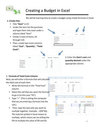
1. Creating a Budget in Excel
We will be learning how to create a budget using simple formulas in Excel.
1. Create lists:
• Title “Item” in C5
• Under the item list the purchase
and type them into excel under a
column titled “Item”.
• Create 5 rows of items, C6
through C10.
• Then, create two more columns
titled “Cost”, “Quantity”, “Total
Costs”.
2. Enter the item’s cost and
quantity desired under the
appropriate column.
3. Formula of Total Costs Column:
Next, we will enter a formula that will calculate
the total cost of each item.
• Write the formula in the “Total Cost”
column.
• Select the cell that you want the formula
to go in (in this case “F6”).
• Type “=” (This is telling the computer
that we are entering a formula into the
cell.)
• Then, type the two cells you want to
multiple together. Example: =(D6*E6).
The asterisk symbol in Excel means to
multiply, which means we are telling the
file to multiply the value of D6 and E6. 1

2.
4. Press the “Enter” key and the file will
multiply the values of the two cells
together.
5. Dragging the formula: Because the
same formula is needed in F7, F8, F9, and
F10, we can drag the formula from F6 into
the other cells.
• Select the cell that contains the
formula you want to drag (in this
case, F6).
• Take your cross hair at the bottom
right hand corner of the cell, click
and drag it down to the last cell you
need the formula to appear. The
formula has been copied to each cell
and will now multiply the values
directly to the left.
6. Gross Cost: Create a cell with the words
“Gross Cost” at the bottom of the chart to
the right.
• In the cell underneath it, type “6% PA
sales Tax”.
• Below that, type “Net Cost”.
2

3. 7. Calculating Gross Cost. The Gross Cost
is the cost of the items minus sales tax
and Shipping and handling. Therefore, we
need to add together the costs of the
items to find out the gross cost.
• Select the cell that you want the
Gross Cost to appear in. Click the
Σ symbol located in the tool bar. A
formula will appear in the cell.
• Highlight the cells you want to add
together (in this case F6‐F10). The
cell names will automatically be put
into the formula. Press enter and
the file will automatically add
together the total cost of your
items.
8. Sales Tax: PA sales tax is 6% or in decimal
form (.06). In order to find what our sales
tax will be, we must multiply our total cost
by 6%.
• Since our total cost appears in cell
“H12”, we need to multiply that cell
by 6%.
• Select the cell you want the sales tax
to appear in. Type “=(“, which again
means that we are typing a formula.
Then, type “=(H12*.06)”. Again, the *
in Excel means multiplication, which
means we are telling the file to
multiply the value of H12 by 6%.
Push “Enter” and the sales tax will
appear in the cell.
3

4. 9. Net Cost: Next, we will total
the “Net Cost”, which is the
total cost including tax.
• Select the cell you want
the Net Cost to appear
in.
• Click the Σ symbol at the
top of the page.
Highlight the cells you
want to add together (in
this case H12‐H13).
• Push “Enter” and the
Net Cost will be
calculated in the cell.
10. Using $ symbol: Lastly, we
need to include the dollar symbol
($) next to all of our money
values.
• Highlight the cells that
contain money values.
• Then click the “$” symbol in
the tool bar above the
document. The values will
then include two decimal
places and the “$” symbol
in front of it.
4