Electrostatics Class 12- Part 3
•Transferir como PPT, PDF•
29 gostaram•13,507 visualizações

![Line Integral of Electric Field (Work Done by Electric Field):
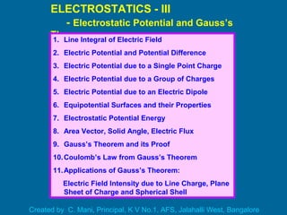
Negative Line Integral of Electric Field represents the work done by the electric
field on a unit positive charge in moving it from one point to another in the
electric field.
+q0
O
Z
Y
X
+ q
F
A
rA
B
rB
r
WAB = dW = - E . dl
A
B
Let q0 be the test charge in place of the unit
positive charge.
The force F = +q0E acts on the test charge
due to the source charge +q.
It is radially outward and tends to accelerate
the test charge. To prevent this
acceleration, equal and opposite force –q0E
has to be applied on the test charge.
Total work done by the electric field on the test charge in moving it from A to B
in the electric field is
=
11qq0
4πε0
][ -
rB rA
WAB = dW = - E . dl
A
B](data:image/gif;base64,R0lGODlhAQABAIAAAAAAAP///yH5BAEAAAAALAAAAAABAAEAAAIBRAA7)
Recomendados
Mais conteúdo relacionado
Mais procurados
Mais procurados (20)
Destaque
Destaque (12)
Semelhante a Electrostatics Class 12- Part 3
Semelhante a Electrostatics Class 12- Part 3 (20)
Mais de Self-employed
Mais de Self-employed (11)
Último
Último (20)
Electrostatics Class 12- Part 3
- 1. ELECTROSTATICS - III - Electrostatic Potential and Gauss’s Theorem1. Line Integral of Electric Field 2. Electric Potential and Potential Difference 3. Electric Potential due to a Single Point Charge 4. Electric Potential due to a Group of Charges 5. Electric Potential due to an Electric Dipole 6. Equipotential Surfaces and their Properties 7. Electrostatic Potential Energy 8. Area Vector, Solid Angle, Electric Flux 9. Gauss’s Theorem and its Proof 10.Coulomb’s Law from Gauss’s Theorem 11.Applications of Gauss’s Theorem: Electric Field Intensity due to Line Charge, Plane Sheet of Charge and Spherical Shell Created by C. Mani, Principal, K V No.1, AFS, Jalahalli West, Bangalore
- 2. Line Integral of Electric Field (Work Done by Electric Field): Negative Line Integral of Electric Field represents the work done by the electric field on a unit positive charge in moving it from one point to another in the electric field. +q0 O Z Y X + q F A rA B rB r WAB = dW = - E . dl A B Let q0 be the test charge in place of the unit positive charge. The force F = +q0E acts on the test charge due to the source charge +q. It is radially outward and tends to accelerate the test charge. To prevent this acceleration, equal and opposite force –q0E has to be applied on the test charge. Total work done by the electric field on the test charge in moving it from A to B in the electric field is = 11qq0 4πε0 ][ - rB rA WAB = dW = - E . dl A B
- 3. 1. The equation shows that the work done in moving a test charge q0 from point A to another point B along any path AB in an electric field due to +q charge depends only on the positions of these points and is independent of the actual path followed between A and B. 2. That is, the line integral of electric field is path independent. 3. Therefore, electric field is ‘conservative field’. 4. Line integral of electric field over a closed path is zero. This is another condition satisfied by conservative field. Note: Line integral of only static electric field is independent of the path followed. However, line integral of the field due to a moving charge is not independent of the path because the field varies with time. E . dl = 0 A B = 11qq0 4πε0 ][ - rB rA WAB = dW = - E . dl A B
- 4. Electric potential is a physical quantity which determines the flow of charges from one body to another. It is a physical quantity that determines the degree of electrification of a body. Electric Potential at a point in the electric field is defined as the work done in moving (without any acceleration) a unit positive charge from infinity to that point against the electrostatic force irrespective of the path followed. Electric Potential: = 11qq0 4πε0 ][ - rB rA WAB = - E . dl A B = 11q 4πε0 ][ - rB rA WAB q0 According to definition, rA = ∞ and rB = r (where r is the distance from the source charge and the point of consideration) = q 4πε0 r W∞B q0 = V V = W∞B q0 SI unit of electric potential is volt (V) or J C-1 or Nm C-1 . Electric potential at a point is one volt if one joule of work is done in moving one coulomb charge from infinity to that point in the electric field. or
- 5. Electric Potential Difference between any two points in the electric field is defined as the work done in moving (without any acceleration) a unit positive charge from one point to the other against the electrostatic force irrespective of the path followed. Electric Potential Difference: = 11qq0 4πε0 ][ - rB rA WAB = - E . dl A B = 11q 4πε0 ][ - rB rA WAB q0 1. Electric potential and potential difference are scalar quantities. 2. Electric potential at infinity is zero. 3. Electric potential near an isolated positive charge (q > 0) is positive and that near an isolated negative charge (q < 0) is negative. 4. cgs unit of electric potential is stat volt. 1 stat volt = 1 erg / stat coulomb or = 11q 4πε0 - rB rA WAB q0 q 4πε0 = VB - VA WAB q0 VB - VA = ∆V =
- 6. Electric Potential due to a Single Point Charge: r + q B x Q ∞ dx q0EE +q0 Let +q0 be the test charge placed at P at a distance x from the source charge +q. To prevent this acceleration, equal and opposite force –q0E has to be applied on the test charge. The force F = +q0E is radially outward and tends to accelerate the test charge. Work done to move q0 from P to Q through ‘dx’ against q0E is dW = F . dx = q0E . dx dW = q0E dx cos 180° = - q0E dx dW = - dx q q0 4πε0 x2 E = q 4πε0 x2 or Total work done to move q0 from A to B (from ∞ to r ) is W∞B = ∞ B dW = - dx q q0 4πε0 x2 ∞ r = - dx q q0 4πε0 x2 ∞ r x2 1 = q 4πε0 r W∞B q0 V = q 4πε0 r P
- 7. Electric Potential due to a Group of Point Charges: +1 C q2 qn q4 P q1 r1 r2 r3r4 rnVP = V1 + V2 + V3 + V4 + …………+ Vn │ │ 1 4πε0 V = ∑ i=1 n qi r - ri ( in terms of position vector ) The net electrostatic potential at a point in the electric field due to a group of charges is the algebraic sum of their individual potentials at that point. 1. Electric potential at a point due to a charge is not affected by the presence of other charges. 2. Potential, V α 1 / r whereas Coulomb’s force F α 1 / r2 . 3. Potential is a scalar whereas Force is a vector. 4. Although V is called the potential at a point, it is actually equal to the potential difference between the points r and ∞. 1 4πε0 V = ∑ i=1 n qi ri q3
- 8. Electric Potential due to an Electric Dipole: ll x P+ q- q p A B +1 C q VP q+ = 4πε0 (x – l) 1 VP = VP q+ + VP q- VP q- = 4πε0 (x + l) 1 - q VP = 4πε0 q (x – l) 1 [ - (x + l) 1 ] VP = 1 4πε0 q . 2l (x2 – l2 ) VP = 1 4πε0 p (x2 – l2 ) i) At a point on the axial line: O
- 9. + q- q p A Bθθ y O ii) At a point on the equatorial line: q VQ q+ = 4πε0 BQ 1 VQ = VP q+ + VP q- VQ q- = 4πε0 AQ 1 - q VQ = 4πε0 q BQ 1 [ - AQ 1 ] VQ = 0 BQ = AQ The net electrostatic potential at a point in the electric field due to an electric dipole at any point on the equatorial line is zero. Q ll
- 10. Equipotential Surfaces: A surface at every point of which the potential due to charge distribution is the same is called equipotential surface. i) For a uniform electric field: E V1 V2 V3 ii) For an isolated charge: E Plane Equipotential Surfaces Spherical Equipotential Surfaces +
- 11. Properties of Equipotential Surfaces: 2. The electric field is always perpendicular to the element dl of the equipotential surface. 1. No work is done in moving a test charge from one point to another on an equipotential surface. WAB q0 VB - VA = ∆V = If A and B are two points on the equipotential surface, then VB = VA . WAB q0 = 0 or WAB = 0 WAB = - E . dl A B = 0 Since no work is done on equipotential surface, i.e. E dl cos θ = 0 As E ≠ 0 and dl ≠ 0, cos θ = 0 or θ = 90°
- 12. 4. Two equipotential surfaces can not intersect. If two equipotential surfaces intersect, then at the points of intersection, there will be two values of the electric potential which is not possible. (Refer to properties of electric lines of force) 3. Equipotential surfaces indicate regions of strong or weak electric fields. dV dr E = - Electric field is defined as the negative potential gradient. or dV E dr = - Since dV is constant on equipotential surface, so E 1 dr α If E is strong (large), dr will be small, i.e. the separation of equipotential surfaces will be smaller (i.e. equipotential surfaces are crowded) and vice versa. Note: Electric potential is a scalar quantity whereas potential gradient is a vector quantity. The negative sign of potential gradient shows that the rate of change of potential with distance is always against the electric field intensity.
- 13. Electrostatic Potential Energy: The work done in moving a charge q from infinity to a point in the field against the electric force is called electrostatic potential energy. W = q V i) Electrostatic Potential Energy of a Two Charges System: O Z Y X A (q1) r1 B (q2) r2 - r1 r2 U = q1q2 4πε 0 │ │- r1 r2 1 or U = q1q2 4πε 0 r12 1
- 14. ii) Electrostatic Potential Energy of a Three Charges System: O Z Y X A (q1) r1 B (q2) r2 or C (q3) r3 - r1r3 - r2r3 U = q1q2 4πε 0 │ │- r1 r2 1 + q1q3 4πε 0 │ │- r1 r3 1 + q2q3 4πε 0 │ │- r2 r3 1 U = q1q2 4πε 0 r12 1 [ q1q3 r31 q2q3 r32 + + ] iii) Electrostatic Potential Energy of an n - Charges System: 1 4πε0 U = ∑ j=1 i≠j n qi qj rj - ri│ │ ∑ i=1 n [2 1 ] - r1r2
- 15. Area Vector: Small area of a surface can be represented by a vector. dS S dS n Electric Flux: Electric flux linked with any surface is defined as the total number of electric lines of force that normally pass through that surface. dS E dS θ 90° θ dS θ dS S Electric flux dΦ through a small area element dS due to an electric field E at an angle θ with dS is = E dS cos θE . dSdΦ = Total electric flux Φ over the whole surface S due to an electric field E is Φ = E . dS S = E S cos θ = E . S dS = dS n Electric flux is a scalar quantity. But it is a property of vector field. SI unit of electric flux is N m2 C-1 or J m C -1 . dS
- 16. Solid Angle: Solid angle is the three-dimensional equivalent of an ordinary two- dimensional plane angle. SI unit of solid angle is steradian. Solid angle subtended by area element dS at the centre O of a sphere of radius r is dΩ = dS cos θ r2 = 4π steradianΩ = dΩ = dS cos θ r2 S S 1. For 0° < θ < 90°, Φ is positive. 2. For θ = 90°, Φ is zero. 3. For 90° < θ < 180°, Φ is negative. Special Cases: r θ dS n r dΩ
- 17. Gauss’s Theorem: The surface integral of the electric field intensity over any closed hypothetical surface (called Gaussian surface) in free space is equal to 1 / ε0 times the net charge enclosed within the surface. E . dS = S ΦE = 1 ε0 ∑ i=1 n qi Proof of Gauss’s Theorem for Spherically Symmetric Surfaces: E . dSdΦ = r2 1 4πε0 = q r . dS n dΦ = r2 1 4πε0 q dS r n. Here, = 1 x 1 cos 0° = 1r n. dΦ = r2 1 4πε0 q dS S ΦE = dΦ r2 1 4πε0 q = 4π r2 ε0 q =dS S r2 1 4πε0 q = O • r r dS E +q
- 18. Proof of Gauss’s Theorem for a Closed Surface of any Shape: EE . dSdΦ = r2 1 4πε0 = q r . dS n dΦ = r2 1 4πε0 q dS r n. Here, = 1 x 1 cos θ = cos θ r n. dΦ = r2 q 4πε0 dS cos θ S ΦE = dΦ q 4πε0 = 4π ε0 q =dΩ q 4πε0 S = dΩ r θ dS n r +q •
- 19. O • r r dS E +q Deduction of Coulomb’s Law from Gauss’s Theorem: From Gauss’s law, E . dS = S ΦE = q ε0 E dS = S ΦE = q ε0 or dS = S ΦE = q ε0 E E = q 4πε0 r2 E x 4π r2 q ε0 = If a charge q0 is placed at a point where E is calculated, then Since E and dS are in the same direction, which is Coulomb’s Law. or F = qq0 4πε0 r2
- 20. Applications of Gauss’s Theorem: 1. Electric Field Intensity due to an Infinitely Long Straight Charged Wire: Gaussian surface is a closed surface, around a charge distribution, such that the electric field intensity has a single fixed value at every point on the surface. From Gauss’s law, E . dS = S ΦE = q ε0 E . dS = S E . dS + A E . dS + B E . dS C E . dS = S E dS cos 90° + A B E dS cos 90° + C E dS cos 0° = C E dS = E x 2 π r l - ∞ + ∞B A C E E E dSdS dS l r
- 21. q ε0 = λ l ε0 (where λ is the liner charge density) E x 2 π r l = λ l ε0 or E = 2 πε0 1 λ r or E = 4 πε0 1 2λ r In vector form, E (r) = 4 πε0 1 2λ r r The direction of the electric field intensity is radially outward from the positive line charge. For negative line charge, it will be radially inward. Note: The electric field intensity is independent of the size of the Gaussian surface constructed. It depends only on the distance of point of consideration. i.e. the Gaussian surface should contain the point of consideration.
- 22. E dS C B A E E dS dS r l 2. Electric Field Intensity due to an Infinitely Long, Thin Plane Sheet of Charge: From Gauss’s law, σ E . dS = S ΦE = q ε0 E . dS = S E . dS + A E . dS + B E . dS C E . dS = S E dS cos 0° + A B E dS cos 0° + C E dS cos 90° = 2E dS = 2E x π r2 TIP: The field lines remain straight, parallel and uniformly spaced.
- 23. (where σ is the surface charge density) or E = 2 ε0 σ In vector form, E (l) = 2 ε0 σ l The direction of the electric field intensity is normal to the plane and away from the positive charge distribution. For negative charge distribution, it will be towards the plane. Note: The electric field intensity is independent of the size of the Gaussian surface constructed. It neither depends on the distance of point of consideration nor the radius of the cylindrical surface. q ε0 = σ π r2 ε0 2 E x π r2 = σ π r2 ε0 If the plane sheet is thick, then the charge distribution will be available on both the sides. So, the charge enclosed within the Gaussian surface will be twice as before. Therefore, the field will be twice. E = ε0 σ
- 24. 3. Electric Field Intensity due to Two Parallel, Infinitely Long, Thin Plane Sheet of Charge: σ1 σ2 E1 E1E1 E2 E2E2 E E E Region I Region II Region III E = E1 + E2 E = 2 ε0 σ1 + σ2 E = E1 - E2 E = 2 ε0 σ1 - σ2 E = E1 + E2 E = 2 ε0 σ1 + σ2 σ1 > σ2 ( ) Case 1: σ1 > σ2
- 25. Case 2: σ1 σ2 E1 E1E1 E2 E2E2 E E E Region I Region II Region III E = E1 - E2 E = 2 ε0 σ1 - σ2 E = E1 + E2 E = 2 ε0 σ1 + σ2 E = E1 - E2 E = 2 ε0 σ1 - σ2 σ1 > σ2 ( ) σ1 > σ2 ( ) + σ1 & - σ2
- 26. Case 3: σ1 σ2 E1 E1E1 E2 E2E2 E = 0 E ≠ 0 Region I Region II Region III E = 0 E = E1 - E2 E = 2 ε0 σ1 - σ2 = 0 E = E1 - E2 E = 2 ε0 σ1 - σ2 = 0 E = E1 + E2 E = 2 ε0 σ1 + σ2 = ε0 σ + σ & - σ
- 27. 4. Electric Field Intensity due to a Uniformed Charged This Spherical Shell: dS E q r R •P From Gauss’s law, E . dS = S ΦE = q ε0 E dS = S ΦE = q ε0 or dS = S ΦE = q ε0 E E x 4π r2 q ε0 = Since E and dS are in the same direction, or E = q 4πε0 r2 i) At a point P outside the shell: Since q = σ x 4π R2 , E = ε0 r2 σ R2 Electric field due to a uniformly charged thin spherical shell at a point outside the shell is such as if the whole charge were concentrated at the centre of the shell. HOLLOW ……… Gaussian Surface O •
- 28. dS EFrom Gauss’s law, E . dS = S ΦE = q ε0 E dS = S ΦE = q ε0 or dS = S ΦE = q ε0 E E x 4π R2 q ε0 = Since E and dS are in the same direction, or E = q 4πε0 R2 ii) At a point A on the surface of the shell: Electric field due to a uniformly charged thin spherical shell at a point on the surface of the shell is maximum. Since q = σ x 4π R2 , E = ε0 σ q R HOLLOW O • •A
- 29. dS E r’ Oq R HOLLOW • B • From Gauss’s law, E . dS = S ΦE = q ε0 E dS = S ΦE = q ε0 or dS = S ΦE = q ε0 E E x 4π r’2 q ε0 = Since E and dS are in the same direction, or E = 0 4πε0 r’2 iii) At a point B inside the shell: This property E = 0 inside a cavity is used for electrostatic shielding. (since q = 0 inside the Gaussian surface) E = 0 r E R O Emax END