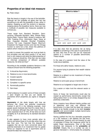
1. Properties of an ideal risk measure
By: Peter Urbani
Risk like beauty is largely in the eye of the beholder.
Although we can probably all agree that risk has
something to do with the possibility of loss, either in
relative- (keeping up with the Jones’s) or absolute-
(keeping above the breadline) terms, there are now
a multitude of possible risk measures available to
confuse you.
These range from Standard Deviation, Semi-
variance, Downside Deviation, Beta, Sharpe Ratio,
Sortino Ratio, Treynor Ratio, Jensen’s measure, M2,
LPM, Tracking Error, Information Ratio, Value at
Risk, Expected Shortfall, Shortfall Probability,
Extreme Tail Loss, Expected Regret, Maximum
Drawdown the Kappa function and now the Omega
function to name but a few. Given this plethora of
options which measure is the best? It is also clear that we perceive risk as being
relative to something in this case A is perceived to
In order to answer this question we must go back to be less risky than B but risk can be measured
first principles and ask what exactly it is we want relative to a number of possible benchmarks.
from a risk measure and what the ideal properties of These include:
such a measure should be. Only then can we make
an informed comparison of different available In the case of a pension fund the value of the
measures. So what are they? funds future liabilities.
According to the available academic literature a risk For those who abhor losses, relative to zero.
measure should have the following properties:
For anyone trying to preserve their wealth relative
1) It should be Asymmetric to inflation.
2) Relative to one or more benchmarks
Relative to a default no-risk investment of having
3) Investor-specific cash in the bank.
4) Multidimensional
Relative to some peer group or benchmark
5) Complete in a specific sense
6) Numerically positive Relative to our budgeted or target rate of return
7) Non-linear For a sector or index fund the relevant sector or
index.
I shall endeavour to explain some of these concepts
in plain English so that you can decide for Some of these risk benchmarks could also be
yourselves which properties you agree or disagree viewed as performance benchmarks except that
with. falling below them is not simply disappointing but
positively undesirable.
Asymmetry of risk deals largely with how we
perceive risk. Given two potential investments Since investors have different liability profiles and
marked A and B in the following example, most or objectives and may use different risk
people would intuitively feel that B is riskier than A. benchmarks it is clear that the ideal risk measure
This is because although they both have the same needs to be flexible enough to be both investor
mean expected return of 10%, B has twice as much specific and accommodate multiple benchmarks
variability as A as denoted by its standard deviation hence multidimensional.
of 10%
Having justified the first four desirable properties
B also appears to have more periods when its of a risk measure I will address the last three,
returns are below those of A and also when they are Completeness, positivity and non-linearity by way
less than zero. The fact that this disquiets us of examples of those risk measures which fail to
suggests that we are more concerned about the satisfy these requirements. One of the more
potential downside of an investment than its upside attractive risk measures is the probability of
hence our response to risk is asymmetric and so shortfall. Clearly this is a number we are in
should the ideal risk-measure be. general interested in. Unfortunately the probability

2. of shortfall measure is not ideal because it is not One of the most widely used measures of risk,
complete. Standard Deviation or Volatility is not really a
measure of risk at all but rather a measure of
If we consider the case of an investor, who is uncertainty. It is also particularly poorly suited for
concerned about losing capital relative to an use as the ideal risk measure for the following
important benchmark and is confronted with two reasons.
hypothetical investment possibilities, E and F. Both
have an expected return of zero relative to the If we consider investments A, C, and D in which both
benchmark and both have a probability of shortfall of C and D have the same standard deviation as one
50%, but are they equally risky? another (10%) whilst A has a standard deviation of
5%. Using standard deviation as your sole measure
If an investors only measure or risk is the shortfall of risk you would be indifferent between C and D.
probability then he/she will be indifferent between E But this is clearly wrong since D has an average
and F. However we can see that F has a greater expected return of -10% versus C’s +10%. Many
potential downside and that everywhere in the people object to standard deviation as a risk
shaded area also a greater probability of realising measure because it gives equal weight to deviations
that downside than E. Thus the shortfall probability above the mean and deviations below the mean,
measure, although interesting, does not address the whereas investors are likely to be more worried
issue of how severe an event may be. It is thus about “downside deviation” than “upside deviation.”
insufficient and incomplete.
Similarly if we now use maximum shortfall as the
only measure of risk using example F and G we can
see although both have the same probability of
shortfall of 50% and the same maximum shortfall of
-30% it is not clear which is riskier because the
maximum shortfall measure alone says nothing
about the size of the typical shortfall. Two
investments may have the same worst outcome but
one may have many large losses and the other only
a few. Information about the end point of the lower
tail of a distribution says little about the distribution
overall. Moreover, we typically have only a few data
points with which to work in the tail making the
maximum shortfall measure both numerically-ill-
conditioned and incomplete as a risk measure.
Another problem with using standard deviation as a
risk measure is that it is not sensitive to order. In the
below examples you can see that A and C have the
same standard deviation and mean.

3. However C is clearly riskier than A, having lost 38% bad as losing half of your money. I don’t think so,”
of its value from its peak to trough during the he says. “It’s at least 10 times as bad.”
hypothetical period shown. Markets that look, or feel, Why VaR is not a coherent measure of risk
volatile often feel that way because of a distinct
order of prices or returns: an order that involves
choppy movements with frequent reversals. This
1) Subadditivity
kind of “order dependent volatility” is not captured by For all random losses X and Y
the technical definition of standard deviation, since p(X)+p(Y) > p(X+Y)
standard deviation is not sensitive to order. This
point has direct application to hedge fund investing, Scenario p(X) p(Y) p(X+Y)
since many hedge fund managers employ trading
strategies whose success or failure will be related
1 0 0 0
not to the volatility of markets but to the path that 2 0 0 0
markets follow 3 0 0 0
4 0 0 0
5 0 0 0
Value at Risk has garnered widespread acceptance
6 0 0 0
in recent years as the new measure of risk. Despite
this widespread use it is also not complete in that it 7 0 0 0
is not mathematically coherent. In order to be 8 0 0 0
mathematically coherent a risk measure must satisfy 9 100 0 100
the conditions of: 10 0 100 100
1.) Subadditivity
2.) Monotonicity VaR @ 85% 0 0 100
3.) Positive Homogeneity and; 0 + 0 is not > 100
4.) Translation invariance.
2) Monotonicity
Without going into detail on these, suffice it to say If X < Y for each scenario then
that Value at Risk fails to satisfy both the
Subadditivity and Monotonicity conditions. This has p(X) < p(Y)
two consequences. The first is that the sum of the
parts may be less than that of the whole and Scenario X Y
secondly that the graphing of value at risk as a 1 1.00 5
function of returns, as in the mean / value at risk 2 2.00 5
frontier, may not result in a neat convex function.
This makes finding the optimal point difficult using 3 3.00 5
conventional methods. 4 4.00 5
5 5.00 5
Fortunately there is one measure of risk, closely 6 5.00 5
related to value at risk that is both mathematically 7 4.00 5
coherent and complete. That is the Expected
Shortfall measure aka. the conditional Value at Risk 8 3.00 5
or Extreme Tail Loss. 9 2.00 5
10 1.00 5
What the Expected Shortfall measure provides is a E( r ) 3.00 5.00
probability weighted average of the expected losses SD 1.41 0.00
in excess of the value at risk. Hence it is the average
of the tail losses conditional on the value at risk
VaR 5.83 5.00
being exceeded. As a risk measure, Expected E( r ) + 2 x SD 5.83 is not < 5
shortfall captures the whole of the downside portion
of the relative probability density function and is
complete. However, its one remaining failing is that 3) Positive Homegeniety
it, like value at risk, is a linear measure of risk.
The non-linearity of risk is closely related to investor For all L > 0 and random losses X
psychology and utility. More people insure their p(L X) = L p(X)
homes than their pets despite the fact that the
possibility of losing a pet is significantly higher than 4) Translation Invariance
losing a home. This reflects the non-linearity of how
we perceive risk. We perceive a low probability of
experiencing a large loss as being far worse than a For all random losses X and constant a
high probability of experiencing a small loss. Frank p(X+a ) = p(X)+a
Sortino says “VaR. It’s simply a linear measure of
risk. It says that losing all your money is twice as

4. Sortino strongly holds the view that it is downside References:
risk that is most important. According to this view,
the most relevant returns are returns below the A unified approach to upside and downside returns
mean, or below zero, or below some other “target” or
– Leslie A Balzar (2001)
“benchmark” return.
This has lead to a proliferation of measures of Expected Shortfall, a natural coherent alternative
“downside risk”: semi-variance, shortfall probability, to Value at Risk - Acerbi and Tasche (2001)
the Sortino ratio, etc. Ignoring the specific
advantages and disadvantages of each individual Coherent measures of risk - Artzner and Delbaen
candidate to represent “the true nature of risk,” we
(1999)
would offer two general observations:
Frequency vs. Amplitude. The idea of risk as
“expected pain” combines two elements: the Peter Urbani, is Head of KnowRisk Consulting. He
likelihood of pain, and the level of pain. The was previously Head of Investment Strategy for
measures described above (with the exception of Fairheads Asset Managers and prior to that Senior
Expected shortfall) focus on one or the other of Portfolio Manager for Commercial Union
these elements, but not both. Semi-variance (and its Investment Management.
descendant, the Sortino ratio) focuses on the size of
the negative surprises, but ignores the probability of He can be reached on (073) 234 -3274
those surprises. Shortfall probability focuses on the
likelihood of falling below a target return, but ignores
the potential size of the shortfall. If I were forced to
pick a single quantitative measure of risk, it would
offer the concept of “expected return below the
target,” defined as the sum of the probability-
weighted below-target returns. This measure is
essentially the area under the probability curve that
lies to the left of the target return level. (Note that
this definition is broad enough to cover both normal
and non-normal distributions.)
Other generalisations of this such as the LPMn
measure and the Omega function which captures
the full distribution are also available.
The final criteria is given as numerical positivity
although this is more a desirable than essential
requirement. Personally I prefer to show loss
percentages such as value at risk in negative terms
since this is more intuitive, but it is more common to
show them +ve because of the widespread use of
quadratic penalties in scientific optimisation.
Past performance does not guarantee anything
regarding future performance, and past risk does not
guarantee anything regarding future risk. This is true
even when the historical record is long enough to
satisfy normal criteria of statistical significance. The
problem is that, just as a performance record is
getting long enough to have statistical significance, it
may no longer have investment significance.
because the people and the organization may have
changed. Investors should thus use the full toolbox
of available risk measures but not loose sight of the
wood for the trees.

5. Useful Calculations in Excel
A B Normal distribution (Prob. density)
0.45
1 Mean 13.13 13.13
2 Std Dev 17.87 0.40
3 CL 0.95 0.35
4 HPR 1 0.30
5 MAR 5.00 0.25
6 0.20
-16.26
7 Normal VaR -16.26
0.15
8 Expected Shortfall -23.73 -23.73
9 Downside Deviation 13.52 0.10
10 Below MAR Deviation 8.53 0.05
11 Shortfall probability 32.46% 0.00
12 Upside Potential 42.52 -60 -40 -20 0 20 40 60 80
13 Average Shortfall -3.79 Normal Probability density Mean is 13.13
14 Upside Potential Ratio 131 Selected probability 5.0% VaR @ 95.0% CL is -16.26
15 Regret 2.24 ETL @ 95.0% CL is -23.73 ABS @ 32.5% CL is 5.00
Normal VaR
=-(-B1*B4-(NORMSINV(1-B3))*B2*SQRT(B4))
Expected Shortfall
=-(-B1*B4+(NORMDIST(NORMSINV(1-
B3),0,1,FALSE)/NORMDIST(NORMSINV(1-B3),0,1,TRUE))*B2*SQRT(B4))
Downside Deviation
=SQRT((((NORMDIST(0,B1,B2,TRUE))*(B2^2+B1^2))-
((B2^2*NORMDIST(0,B1,B2,FALSE))*B1))/NORMDIST(0,B1,B2,TRUE))
Below MAR Deviation
=SQRT(((B5-B1)^2+B2^2)*NORMDIST(B5,B1,B2,TRUE)+(B5-
B1)*NORMDIST(B5,B1,B2,FALSE)*B2*B2)
Shortfall probability
=NORMDIST(B5,B1,B2,TRUE)
Upside Potential
=-(-B1*B4-(NORMSINV(B3))*B2*SQRT(B4))
Average Shortfall
=-((B5-B1)*NORMDIST(B5,B1,B2,TRUE)+NORMDIST(B5,B1,B2,FALSE)*B2*B2)
Upside Potential Ratio
=B12/B11
Regret
=((NORMDIST(B5,B1,B2,TRUE)*(B2^2+B1^2-2*B5*B1+B5^2))-
((NORMDIST(B5,B1,B2,FALSE)*B2^2)*(B1-B5)))/NORMDIST(B5,B2,B3,TRUE)/100