An optical time-domain reflectometer (OTDR) is an optoelectronic instrument used to characterize an optical fiber. An OTDR is the optical equivalent of an electronic time domain reflectometer. It injects a series of optical pulses into the fiber under test and extracts, from the same end of the fiber, light that is scattered (Rayleigh backscatter) or reflected back from points along the fiber. The scattered or reflected light that is gathered back is used to characterize the optical fiber. This is equivalent to the way that an electronic time-domain meter measures reflections caused by changes in the impedance of the cable under test. The strength of the return pulses is measured and integrated as a function of time, and plotted as a function of fiber length.

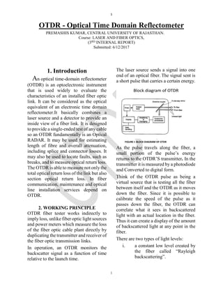
1. 1
1
OTDR - Optical Time Domain Reflectometer
PREMASHIS KUMAR, CENTRAL UNIVERSITY OF RAJASTHAN.
Course: LASER AND FIBER OPTICS,
(3RD INTERNAL REPORT)
Submitted: 6/12/2017
1. Introduction
An optical time-domain reflectometer
(OTDR) is an optoelectronic instrument
that is used widely to evaluate the
characteristics of an installed fiber optic
link. It can be considered as the optical
equivalent of an electronic time domain
reflectometer.It basically combines a
laser source and a detector to provide an
inside view of a fiber link. It is designed
to provide a single-ended test of any cable
so an OTDR fundamentally is an Optical
RADAR. It may be used for estimating
length of fibre and overall attenuation,
including splice and connector losses. It
may also be used to locate faults, such as
breaks, and to measure optical return loss.
The OTDR is able to measure not only the
total optical return loss of the link but also
section optical return loss. In fiber
communication, maintenance and optical
line installation services depend on
OTDR.
2. WORKING PRINCIPLE
OTDR fiber tester works indirectly to
imply loss, unlike fiber optic light sources
and power meters which measure the loss
of the fiber optic cable plant directly by
duplicating the transmitter and receiver of
the fiber optic transmission links.
In operation, an OTDR monitors the
backscatter signal as a function of time
relative to the launch time.
The laser source sends a signal into one
end of an optical fiber. The signal sent is
a short pulse that carries a certain energy.
FIGURE I: BLOCK DIAGRAM OF OTDR
As the pulse travels along the fiber, a
small portion of the pulse’s energy
returns to the OTDR’S transmitter. In the
transmitter it is measured by a photodiode
and Converted to digital form.
Think of the OTDR pulse as being a
virtual source that is testing all the fiber
between itself and the OTDR as it moves
down the fiber. Since it is possible to
calibrate the speed of the pulse as it
passes down the fiber, the OTDR can
correlate what it sees in backscattered
light with an actual location in the fiber.
Thus it can create a display of the amount
of backscattered light at any point in the
fiber.
There are two types of light levels:
i. a constant low level created by
the fiber called “Rayleigh
backscattering”.

2. Optical Time domain Reflectometer
2
ii. a high-reflection peak at the
connection points called
“Fresnel reflection”.
Rayleigh backscattering is used to
calculate the level of attenuation in the
fiber. This phenomenon comes from the
natural reflection and absorption of
impurities inside optical fiber. As the
light is scattered in all directions, some of
it just happens to return back along the
fiber towards the light source.
FIGURE II: BACKSCTTERING IN OTDR
Higher wavelengths are less attenuated
than shorter ones and, therefore, require
less power to travel over the same
distance in a standard fiber.
The second type of reflection used by an
OTDR—Fresnel reflection—detects
physical events along the link. When the
light hits an abrupt change in index of
refraction (e.g., from glass to air) a higher
amount of light is reflected back, creating
Fresnel reflection, which can be
thousands of times bigger than the
Rayleigh backscattering. Fresnel
reflection is identifiable by the spikes in
an OTDR trace. Examples of such
reflections are connectors, mechanical
splices, bulkheads, fiber breaks or opened
connectors.
3. MATHEMATICAL FORMULAE
There are some calculations involved.
As the light has to go out and come back,
so we have to factor that into the time
calculations, cutting the time in half and
the loss calculations, since the light sees
loss both ways. The power loss is a
logarithmic function, so the power is
measured in dB.
The location of any event in OTDR can
be figure out by using the equation given
below:
Distance, Z=
.
t: two-way propagation delay time
v: velocity of light in the fiber
Its known that the light intensity in the
fiber in the function of the distance is the
following:
where α= + , the sum of
the scattering and absorption losses in
dB/km.
The total scattered power at distance of
z:
(z) = Δz (z)
Where:
Δz , impulse length in the fiber,
, scattering loss, given in ratio/km.
Since the numerical aperture of the fiber
is finite, only a certain part of the
scattered light can travel backward in the
fiber(S).This also faces losses during the
propagation in the fiber and it reaches
the input of the fiber, where the total
backscattered power is:
(z) = Δz 10 )
S= /4.55 in case of a single mode
fiber

3. Optical Time domain Reflectometer
3
The directly measured loss is then halved
electronically before plotting the output
trace.
4. OTDR BASIC PARAMATER
OTDR user is required to key in these
four basic data parameters into OTDR in
order to get good and accurate fiber
trace analysis:
A. Dynamic Range
B. Pulse Width
C. Index of Refraction
D. Averaging Time
Dynamic Range
An important OTDR
parameter is the dynamic range. It is the
maximum length of fiber that the longest
pulse can reach. Therefore, the bigger the
dynamic range (in dB), the longer the
distance reached. Using the proper
distance range is the key to increasing the
maximum measurable distance. A good
rule of thumb is to choose an OTDR that
has a dynamic range that is 5 to 8 dB
higher than the maximum loss that will be
encountered. The more loss there is in the
network, the more dynamic range will be
required.
PULSE WIDTH
The pulse width is time
during which the
FIGURE III: PULSE WIDTH OF OTDR
Laser is on. Time is converted into
distance so that the pulse width has a
length.
Longer pulse widths are used for longer
range tests. As distance increases, pulse
width must go up, otherwise traces will
appear “noisy” and rough. However, dead
zones extend along with the pulse width.
Pulse width also decides the resolution of
optical fiber.
Index of Refraction
Index of Refraction
is a way of measuring the speed of light
in a material. Light travels fastest in a
vacuum and Index of Refraction is
calculated by dividing the speed of light
in a vacuum by the speed of light in core
medium. If the Group Index of Refraction
(GIR) setting in the OTDR does not match
that of the fiber under test, the results
will show incorrect distances.
Averaging Time
We can consider
averaging time as the time taken to have
good OTDR trace.
OTDRs can take multiple samples of the
trace and average the results. Averaging
time refers to how long the user allows
the device to take samples.

4. Optical Time domain Reflectometer
4
The longer the averaging time is allowed,
the better will be the result. Eventually,
enough data is averaged for a good test
and continuing to test won’t yield any
more of an accurate result.
The two traces pictured here were
captured from the same cable plant with
all of the same settings except for the
number of averages. The first trace is
only one test, while the second one is
averaged from 1024 pulses.
We can observe the difference in the
distance that the signal travels before it
the noise level becomes significant.
5. EVENTS IN OTDR TRACES
Trace of OTDR is a visual representation
of the backscattering coefficient.The
slope of the trace shows the attenuation
coefficient of the fiber and is calibrated in
dB/km by the OTDR. “Trace” takes a lot
of words to describe all the information in
it.
Decaying signal associated with the fiber
losses.
FIGURE 4: TRACE OF OTDR
Small but finite drops in the backscatter
signal on the trace corresponds to losses
due to the presence of non-reflective
elements-Fused coupler, tight bends,
thermal splices.
But connectors and mechanical splices
will show a reflective peak. The height of
that peak will indicate the amount of
Fresnel reflection at the event, unless it is
so large that it saturates the OTDR
receiver.
An abrupt drop in the background signal
corresponds to interruptions at
connectors, non-fiber components and
termination of fiber.
These features of the trace is called
‘events’ in OTDR jargon.
Most commonly, users manipulate two
cursors, “A” and “B”, to illustrate what is
referred to as “two point loss” on an
OTDR result.
This can be used to show loss in a single
event or in a group of events. These
cursors can be individually moved left
and right to specific points on the result.
6. Reliability and quality of OTDR
equipment
Some of the terms often used in
specifying the quality of an OTDR are as
follows:
Accuracy: Defined as the correctness of
the measurement i.e., the difference
between the measured value and the true
value of the event being measured.
Measurement range: Defined as the
maximum attenuation that can be placed
between the instrument and the event
being measured, for which the instrument
will still be able to measure the event
within acceptable accuracy limits.
Spatial Resolution: It is one of the key
performance features of an OTDR. It is
Minimum separation at which two events
can be distinguished. It depends on pulse

5. Optical Time domain Reflectometer
5
width.
FIGURE 5: RESOLUTION OF OTDR
While the longer pulses yield traces with
less noise and longer distance capability,
the ability to resolve and identify events
becomes less.
7. Dead Zones
Large Fresnel reflection signals can cause
problems for the detection system
transient but strong saturation of the front
end receiver. The length of the fiber
masked in terms of event detection by this
way is known as a Dead Zone. The length
of Dead Zone is determined by the pulse
width.
Dead zones that is arising from fiber input
is called near end dead zone and dead
zones arising from fiber output is called
far end dead zones.
FIGURE 6: DEAD ZONE OF OTDR TRACE
Strong Fresnel reflections give rise to
dead zones of the order of hundreds of
meters is corresponding to detector
recovery periods of many tens of receiver
time constant.
Many OTDRs incorporate a dead zone
masking feature- selectively attenuate
large incoming reflected signal pulses .
Near end dead zone and event dead zones
present greater problems in shorter
networks.
In OTDR trace there is two types of dead
zone:
i. Event Dead Zone: Refers to the
minimum necessary for
consecutive reflection events can
be "solved", i.e differentiated from
each other.
ii. Attenuation Dead Zone: Refers to
the minimum required distance
after a reflective event, for the
OTDR to measure a loss of
reflective event or reflection.
8. Ghosts
When we are testing short cables with
highly reflective connectors we normally
encounter “ghosts.” Ghost is Caused by
the reflected light from the far end
connector reflecting back and forth in the
fiber until it is attenuated to the noise
level. Ghost in trace of OTDR is Very
confusing, as they seem to be real
reflective events like connectors.
FIGURE 7:GHOST IN OTDR TRACE
Ghosts normally arrive multiples of the
length of the launch cable or the first

6. Optical Time domain Reflectometer
6
cable. Ghosts in trace of OTDR Can be
eliminated by reducing the reflections
using index matching fluid on the end of
the launch cable.
9. Discussion
OTDR is the Industry standard for
measuring Loss characteristics of a link
or network, monitoring the network
status and locating faults and degrading
components. OTDR tests are often
performed in both directions and the
results are averaged, resulting in bi-
directional event loss analysis.
The limited distance resolution of the
OTDR makes it very hard to use in a LAN
or building environment where cables are
usually only a few hundred meters long.
The OTDR has a great deal of difficulty
resolving features in the short.
Acknowledgements: I would like to
thank our course instructor
DR.RAJNEESH KUMAR VERMA.
References
[1]TATEDA, MITSUHIRO;
HORIGUCHI,TSUNEO; “Advances in
Optical Time-Domain Reflectometry”
[2] Hartog, Arthur; "Optical time domain
reflectometry”
[3]http://www.thefoa.org/tech/ref/testing/OT
DR/OTDR.html
[4]https://www.techopedia.com/definition/2
621/optical-time-domain-reflectometer-otdr
[5]http://www.exfo.com/glossary/optical-
time-domain-reflectometer-otd
[6]https://en.wikipedia.org/wiki/Optical_time
-domain_reflectometer
[7]https://www.fs.com/optical-time-domain-
reflectometer-tutorial-aid-387.html