Automatic differentiation, specializing in compiler technology, parallel network computing, numerical methods and discrete algorithms.

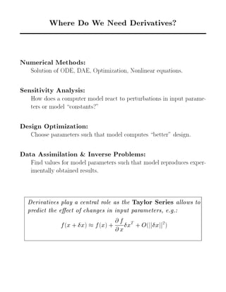
1. Where Do We Need Derivatives?
Numerical Methods:
Solution of ODE, DAE, Optimization, Nonlinear equations.
Sensitivity Analysis:
How does a computer model react to perturbations in input parame-
ters or model constants?"
Design Optimization:
Choose parameters such that model computes better" design.
Data Assimilation & Inverse Problems:
Find values for model parameters such that model reproduces exper-
imentally obtained results.
Derivatives play a central role as the Taylor Series allows to
predict the eect of changes in input parameters, e.g.:
f(x + x) f(x) +
@ f
@ x
xT + O(jjxjj2)

2. Approaches to Computing Derivatives
By Hand:
Tedious and Error-Prone
Divided Dierences:
Can't assess reliability. Dicult to assess numerical accuracy (e.g.,
truncation and cancellation error) and expensive when computing
derivatives w.r.t. many independent variables.
one-sided dis:
@ f(x)
@ xi
jx=xo
f(xo h ei) f(xo)
h
central dis:
@ f(x)
@ xi
jx=xo
f(xo + h ei) f(xo h ei)
2h
Symbolic:
Infeasible for large codes. Not directly applicable to larger programs
with loops and branches. (e.g., Maple, Mathematica)
Automatic Dierentiation:
Requires little human time
Incurs no truncation error
Attractive computational complexity
Applicable to codes of arbitrary size

3. Hierarchical Structure of ADIFOR
Lots of
Alternatives
Program
Procedure
Loop Nest
Loop Body
Basic Block
Statement
Expression
ADIFOR Approach

4. Fortran
Analysis
Code
AD Intrinsics
Template
Expander
Fortran
Derivative
Code
Derivative
Computing
Code
The ADIFOR System
ADIFOR
Preprocessor
Compile
and Link
AD Intrinsics
Library
User’s
Derivative
Driver
SparsLinC
Library
Computational Differentiation
at Argonne National Laboratory

5. ODE’s, DAE’s
Optimization
Iterative
Solvers
C, C++
Fortran
(77,90,M,HPF)
MPI,PVM
Little
Languages
The Big Picture of AD Tools
Hessians
Non-smooth functions
New
Capabilities
New
Languages
Chain
Rule
Numerical
Methods
Associativity
Pseudo-Adjoints, Interface
Contraction, Breaking Dependencies

6. A Modular Approach to Building AD Tools
Input Program
Parsing and Canonicalization Program Analysis
Annotated
Intermediate Representation
Differentiation Executive
Derivative Augmentation
Unparsing
Parallel Output Program
Parallel
Derivative
Run-time
System

7. Time-Parallel Scheme for Derivative Computing
(FORTRAN-M Implementation)
Chain rule associativity breaks dependencies and generates new
task parallelism (in addition to existing one!).
x y
Ht Ht+1
dH t /dx dH t + 1 /dy dH t + 2 /dz
... Serial top-level
Manager
parallel_to_MM channel
Matrix-matrix
Master Wrapper
Multiplier
parallel_to_MM channel
Gradient Process 1
manager_to_parallel channel
manager_to_parallel channel
idle channel
idle channel
Gradient Process N
serial_to_manager channel
w
y z
z
x
y
dw/dx
proc. 0
proc. 1
proc. 2
Compute_Der Compute_Fun Compute_Mat Receive Send
7 22 36 50 65 79 94
0
1
2
3
4
5
6
7
8

8. Time-Parallel Scheme for Derivative Computing
(MPI Implementation)
Chain rule associativity breaks dependencies and generates new
task parallelism (in addition to existing one!).
x y Ht Hy t+1
x y
x Ht H z t+1
dH t /dx dH t + 1 /dy dH t + 2 /dz
dw/dx
w
proc. 0
proc. 1
proc. 2
y z
Master Wrapper
Manager
(option)
Gradient Process 1
Matrix-matrix
Multiplier
Gradient Process N
parallel_to_MM channel
parallel_to_MM channel
manager_to_parallel channel
manager_to_parallel channel
idle channel
idle channel
...
Compute_Der Compute_Fun Compute_Mat Receive Send
3.0 9.1 15.1 21.2 27.2 33.3 39.3
0
1
2
3
4
5
6
7
8
9

9. Parallel System Design with Task Manager
The parallel-task manager process will keep track of which pro-
cesses are active, and select an inactive process and send an
activations message to that process. This allows for a het-
erogeneous compute situation, where we might have a slower
processor.
Compute_Der Compute_Fun Compute_Mat Receive Send
4.9 14.6 24.3 34.0 43.7 53.4 63.1
0
1
2
3
4
(System Design without Task Manager)
Compute_Der Compute_Fun Compute_Mat Receive Send
5.0 15.0 25.0 35.0 45.0 55.0 65.0
0
1
2
3
4
5
(System Design with Task Manager)
For the parallel resource utilization, spawning parallel gradi-
ents computing can be done either by the round-robin scheme
statically (top), or by introducing a task manager dynamically
(bottom).

10. Parallel System Design with Task Manager
The parallel-task manager process will keep track of which pro-
cesses are active, and select an inactive process and send an
activations message to that process. This allows for a het-
erogeneous compute situation, where we might have a slower
processor.
Compute_Der Compute_Fun Compute_Mat Receive Send
4.2 12.5 20.8 29.1 37.4 45.7 54.0
0
1
2
3
4
(System Design without Task Manager)
Compute_Der Compute_Fun Compute_Mat Receive Send
4.2 12.6 21.0 29.4 37.8 46.2 54.6
0
1
2
3
4
5
(System Design with Task Manager)
For the parallel resource utilization, spawning parallel gradi-
ents computing can be done either by the round-robin scheme
statically (top), or by introducing a task manager dynamically
(bottom).

11. Upshot: Parallel Performance Analysis
Compute_Der Compute_Fun Compute_Mat Receive Send
64 191 319 446 573 701 828
0
1
2
3
4
(ADIFOR Dense)
Compute_Der Compute_Fun Compute_Mat Receive Send
65 196 326 457 587 717 848
0
1
2
3
4
(ADIFOR Color)
Compute_Der Compute_Fun Compute_Mat Receive Send
76 228 380 533 685 837 989
0
1
2
3
4
(ADIFOR Sparse)
Compute_Der Compute_Fun Compute_Mat Receive Send
76 227 378 529 680 831 982
0
1
2
3
4
(ADIFOR Mixed-1)
Compute_Der Compute_Fun Compute_Mat Receive Send
94 283 471 659 848 1036 1224
0
1
2
3
4
(ADIFOR Mixed-2)

12. Speedup for ADIFOR Application:
Shallow Water Equations model (SWE)
The serial and parallel speedup for the ShallowWater Equations
model (SWE), which utilizes a time-dependent leapfrog scheme.
Shallow Water Equations model (SWE)
grid size = 21x21 n = 3*21*21 = 1323, p = 4, s = n + p = 1327
machine: IBM SP, time-loop: 40
160.00
140.00
120.00
100.00
80.00
60.00
40.00
20.00
0.00
ADIFOR Serial Parallel: 1 2 4 8 16 32
no. of derivative slaves
Speedup
Dense
Color
Sparse
Mixed-1
Mixed-2
The serial speedup has been done by employing the chain rule
and the sparsity patterns. Chain rule associativity breaks de-
pendencies and generates new task parallelism.

13. ADIFOR Application:
Shallow Water Equations model (SWE)
The Shallow Water Equations model (SWE), which utilizes a
time-dependent leapfrog scheme.
We let Z(t); Z(t 1) denote the current and previous state of
the time-dependent system. The next state is obtained by
Z(t + 1) = G(Z(t); Z(t + 1);W;B(t + 1);Obs(t + 1))
where G is the time-stepping operator, W are the time-
independent parameters, B(t + 1) are the next boundary con-
ditions, and Obs(t + 1) are observations of the next state.
0
5
10
15
20
25
0
5
10
15
20
20
10
0
−10
−20
−30
−40
−50
25
Shallow Water Equations model (SWE)
0
5
10
15
20
25
0
5
10
15
20
4
2
0
−2
−4
−6
−8
−10
25
x 106
Shallow Water Equations model (SWE) AD−Sensitivity
4-D variational data assimilation with shallow water equations
(SWE) when controlling both boundary and initial conditions
(left) and its sensitivity to a uniform relative change in the
observations and weights (right).

14. ADIFOR Application: MM5 PSU/NCAR
Mesoscale Weather Model
The Fifth-Generation Penn State/NCAR Mesoscale Weather
Model (MM5) is regional forecasting model. See A Description
of the Fifth-Generation Penn State/NCAR Mesoscale Weather
Model (MM5), G. A. Grell, J. Dudhia, and D. R. Stauer,
NCAR/TN-398+STR, 1994.
Water vapor mass fraction (left) and its sensitivity to a uniform
relative change in the surface pressure

15. eld (right).

16. MM5's Sensitivity to Initial Temperature
Grid size: 63 63 23.
Median distance of grid points: 101 km.
Radius of perturbation: 4.6 grid points.
Sensitivity of Temperature in deg/deg at
time t = 0h 30min (6th time step) on the
519 mb sigma-level.

17. ADIFOR Application:
High-Speed Civil Transport
MARSEN: 3-D marching Euler code - Vamshi Mohan Ko-
rivi and Art Taylor, Old Dominion University, Perry Newman,
NASA Langley
Aerodyn. Opt. Studies using a 3-D Supersonic
Euler Code with Ecient Calculation of Sensi-
tivity Derivatives, V. M. Korivi, P. Newman, A.
Taylor, AIAA-94-4270-CP, 1994.