SlideShare uma empresa Scribd logo
1 de 33
Bulletin of Mathematical Biology (2007) 69: 1199–1231
DOI 10.1007/s11538-006-9130-8

ORIGINAL ARTICLE


Chemical Organisation Theory

Peter Dittrich∗ , Pietro Speroni di Fenizio

Bio Systems Analysis Group, Jena Centre for Bioinformatics and Department
of Mathematics and Computer Science, Friedrich Schiller University Jena,
D-07743 Jena, Germany

Received: 14 February 2005 / Accepted: 29 March 2006 / Published online: 6 April 2007
C Society for Mathematical Biology 2007


Abstract Complex dynamical reaction networks consisting of many components
that interact and produce each other are difficult to understand, especially, when
new component types may appear and present component types may vanish com-
pletely. Inspired by Fontana and Buss (Bull. Math. Biol., 56, 1–64) we outline a
theory to deal with such systems. The theory consists of two parts. The first part
introduces the concept of a chemical organisation as a closed and self-maintaining
set of components. This concept allows to map a complex (reaction) network to
the set of organisations, providing a new view on the system’s structure. The sec-
ond part connects dynamics with the set of organisations, which allows to map a
movement of the system in state space to a movement in the set of organisations.
The relevancy of our theory is underlined by a theorem that says that given a dif-
ferential equation describing the chemical dynamics of the network, then every
stationary state is an instance of an organisation. For demonstration, the theory
is applied to a small model of HIV-immune system interaction by Wodarz and
Nowak (Proc. Natl. Acad. USA, 96, 14464–14469) and to a large model of the
sugar metabolism of E. Coli by Puchalka and Kierzek (Biophys. J., 86, 1357–1372).
In both cases organisations where uncovered, which could be related to functions.

Keywords Reaction networks · Constraint based network analysis · Hierarchical
decomposition · Constructive dynamical systems

1. Constructive dynamical systems

Our world is changing, qualitatively and quantitatively. The characteristics of its
dynamics can be as simple as in the case of a friction-less swinging pendulum,
or as complex as the dynamical process that results in the creative apparition of


Both authors contributed equally.
∗ Corresponding  author.
E-mail address: dittrich@minet.uni-jena.de (Peter Dittrich).
1200                                                            Dittrich and di Fenizio


novel ideas or entities. We might characterise the nature of a dynamical process
according to its level of novelty production. For example, the friction-less swinging
pendulum implies a process where the novelty is only quantitative. Whereas the
process of biological evolution is highly creative and generates qualitative novel-
ties, which then spread in a quantitative way.
   Fontana and Buss (1994) called processes and systems that display the produc-
tion of novelty, constructive (dynamical) processes and constructive (dynamical)
systems, respectively. Constructive systems can be found on all levels of scientific
abstraction: in nuclear physics, where the collision of atoms or subatomic particles
leads to the creation of new particles; in molecular chemistry, where molecules can
react to form new molecules; or in social systems, where communication can lead
to new communication (Luhmann, 1984). As a result of a combinatorial explosion,
it is easy to create something that is new, e.g. a molecule or a poem that is unique
in the whole known universe.
   Despite the fact that a large amount of interesting dynamical processes are con-
structive, classical systems theory does not, conveniently, take novelty into ac-
count. Classical systems theory assumes a given static set of components (Murray,
2004; Heij et al., 2006). For example, a classical systems analysis would first iden-
tify all components and their relations; then would identify a state space with fixed
dimensionality, and then study the behaviour of the system in such space. For ex-
ample to study a pendulum a scientist would describe its state as specified by angle,
radius, and angular velocity and plot the orbit in that state space.
   This kind of analysis assumes that all components are always present in the sys-
tem, and the change in time will mainly be a changed in the relative amount, thus a
quantitative change. What we claim here is that this represents only a tiny percent-
age of systems, but for the great majority new object are produced. A simple exam-
ple would be any natural system that evolves. Not only new objects are produced
but objects previously present diminish in quantity and eventually disappear. Thus
the movement is not so much a quantitative movement in the fixed state space,
but a qualitative movement that goes from state space to state space, as new ob-
jects appear and old objects disappear. Following Fontana and Buss (1994) we will
refer in this paper to the theory necessary to study such systems as constructive
dynamical system theory.
   The lack of a theory for constructive dynamical systems has been presented,
identified and discussed in detail by Fontana and Buss (1994) in the context of a
theory for biological organisation. As a partial solution, they suggested the impor-
tant concept of a (biological) organisation as a set of objects (molecules in that
context) algebraically closed and dynamically self-maintaining. Before we define
a (chemical) organisation precisely in Section 2.3, we give a brief overview of the
concept, here.
   An organisation is defined as a set of objects that is closed and self-maintaining.
Closure means that no new object can appear because of the interaction within the
set (Section 2.2.1). As such no novelty can spontaneously appear. Self-maintaining
means that every consumed object of the set has a way to be generated within the
set so that it does not disappear from the system (Section 2.3.1). Although those
two properties do not assure that a set of objects will remain unchanged in time,
the lack of them does imply that the system will eventually qualitatively move to
Chemical Organisation Theory                                                      1201


a different set of objects (Section 3.2). In a vast class of systems, which we call
consistent (Section 2.4), it is possible to define a generator operator such that from
any set of objects an organisation is uniquely defined. The organisation generated
by a set A represents the largest possible set of objects that can stably exists when
starting with A. This implies that the set of all organisations partitions the set of
all possible sets of objects. Thus, as the system qualitatively progress from one set
to another we can follow it on the more tractable set of all possible organisations
(Section 3.3). The study of this movement together with a theorem relating fixed
points to organisations will be the core concepts of Section 3, where the dynamical
analysis is presented.

1.1. Reaction systems

The theory described herein aims at understanding reaction systems. A reaction
system consists of objects, and interaction rules among objects that lead to the
appearance or disappearance of other objects.
   Reaction systems are not used only to model chemical phenomena. Their ap-
plications range from ecology (Schuster and Sigmund, 1983), proto-biology (Segre      ´
et al., 1998), systems biology (Puchalka and Kierzek, 2004), bioinformatics to com-
                      ˆ          ´
puter science (Banatre and Metayer, 1990) and reach even the study of language
and social systems (Dittrich et al., 2003). For this reason the same concept took
different labels in different context. What gets referred to as a ‘species’ in ecology
might be referred as a ‘molecule’ in chemistry, as a ‘word’ in study of language, as
                                            ˆ           ´
a ‘token’ (Petri, 1962) or ‘process’ (Banatre and Metayer, 1990) in computer sci-
ence, and as a ‘cultural meme’ or ‘communication’ in sociology (Luhmann, 1984).
All this refers to the same concept: objects, that through the reaction laws generate
other objects. Instead of using always the neutral and vague term ‘object,’ in this
paper, we will use a series of terms as absolutely equivalent: ‘molecule,’ ‘molecular
species,’ or simply ‘species’. While we will avoid to use the (too context specific)
terms like ‘language’ or ‘word.’ The interaction among molecules that lead to the
appearance or disappearance of molecules will be called a reaction.
   Note that we have to distinguish between a reaction system as an abstract de-
scription of all possible molecules (and their reactions), and an actual reaction
vessel, which contains concrete instances of molecules from the set of all possible
molecules.
   As we will see in the course of this paper, the description of a reaction system can
be subdivided into three parts: (1) the set of all possible molecules M, (2) the set
of all possible reactions among all the possible molecules R, and (3) the dynamics
(e.g. kinetic laws), which describes how the reactions are applied to a collection
                                                   ´           ´
of molecules inside a reaction vessel (see e.g. Erdi and Toth, 1989; Heinrich and
Schuster, 1996).


2. Static analysis

In the first part of the paper (Section 2), we are only concerned with the static struc-
ture of a reaction system, that is, the molecules M and the reactions R. Instead of
1202                                                                          Dittrich and di Fenizio


considering a state, e.g. a concentration vector, we limit ourself to the analysis of
the set of molecules present in that state.

2.1. Algebraic chemistry

We introduce the concept of an algebraic chemistry, which effectively is the re-
action network (including stoichiometric information), but that neglects the dy-
namics (kinetic laws). The algebraic chemistry represents the required input data
structure, from which we will derive the organisational structure of the reaction
system.
   In this work we will refer often to multisets. A multiset is a collection of ob-
jects such that each object can appear with a multiplicity higher than 1. As such a
multiset is essentially a set where the same object can appear more than one time.
Generally the frequency of occurrence of an element a in a multiset A is denoted
by #(a ∈ A). Also given a set C we will also refer to PM (C) as the set of all multisets
with elements from C.

Definition 1 (algebraic chemistry). Given a set M of elements, called molecules,
and a set of reaction rules R given by the relation R : PM (M) × PM (M). We call
the pair M, R an algebraic chemistry.

   For simplicity, we adopt the notation from chemistry to write reaction rules. In-
stead of writing ({s1 , s2 , . . . , sn }, {s1 , s2 , . . . , sn }) ∈ R we write: s1 + s2 + · · · + sn →
s1 + s2 + · · · + sn . Given the left hand side molecules A = {s1 , s2 , . . . , sn } and the
right hand side molecules B = {s1 , s2 , . . . , sn }, we write (A → B) ∈ R instead of
(A, B) ∈ R. A → B represents a chemical reaction equation where A is the multi-
set of molecules on the left hand side (also called reactants) and B the multiset of
molecules on the right hand side (also called products).

2.1.1. Input and output
There are many processes that give rise to an inflow and outflow, such as, incident
sunlight, decaying molecules, or a general dilution flow. In this paper we interpret
the reaction rule ∅ → a as an input of a, and a → ∅ as an output of a (∅ denoting
the empty set). In the example that follows (Fig. 1) b, c and d decay spontaneously.

Example 2. (algebraic chemistry). In this paper we will illustrate the new con-
cepts using a small example where there are just four molecular species M =
{a, b, c, d}, which react according to the following reaction rules R = {a + b →
a + 2b, a + d → a + 2d, b + c → 2c, c → b, b + d → c, b → ∅, c → ∅, d → ∅}. A
graphical representation of this reaction network can be found in Fig. 1.


2.2. Semi-organisation:= closed and semi-self-maintaining set

In classical analysis, we study the movement of the system in state space. Instead,
here, we consider the movement from one set of molecules to another. As in the
Chemical Organisation Theory                                                                  1203


Fig. 1 Example with four species. Reaction network (a ‘2’ means that two molecules are pro-
duced) and graphical representation of the lattice of all sets. The vertical position is determined
by the set size. The solid lines depict the lattice of organisations.

classical analysis of the dynamics of the system, where fixed points and attractors
are considered more important than other states, some sets of molecules are more
important than others. In order to find those sets, we introduce some properties
that define them, namely: closure, semi-self-maintenance, semi-organisation, self-
maintenance, and finally being an organisation. All definitions herein refer to an
algebraic chemistry M, R .

2.2.1. Closed sets
The first requirement, called closure, assures that a no new molecule can be gen-
erated by the reactions inside a set or equivalently that all molecules that can be
generated by reactions inside a set are already inside the set

Definition 3 (closed set). A set C ⊆ M is closed, if for all reactions (A → B) ∈
R, with A a multiset of elements in C (A ∈ PM (C)), then B is also a multiset of
elements in C (B ∈ PM (C)).

  Given a set S ⊆ M, we can always generate its closure GCL (S) according to the
following definition:

Definition 4 (generate closed set). Given a set of molecules S ⊆ M, we define
GCL (S) as the smallest closed set C containing S. We say that S generates the closed
set C = GCL (S) and we call C the closure of S.
1204                                                                     Dittrich and di Fenizio


  We need to prove that this definition is unambiguous: Let us suppose, ad
absurdum, that we can find two smaller closed sets U, V with S ⊆ U, V and U = V.
Since the intersection of closed sets is trivially closed, so U ∩ V would be closed
too but S ⊆ U ∩ V. Thus, we have found a closed set smaller than U and V that
contains S, against the supposition.
Example 5 (closed sets). In our example test bed (Example 2) there are 10 closed
sets: {}, {a}, {b}, {d}, {a, b}, {b, c}, {a, d}, {a, b, c}, {b, c, d} and {a, b, c, d}. The empty
set is closed, because there is no input. If there would be an input, the smallest
closed set would be the closed set generated from the input set. Assume, for exam-
ple, that the reaction rule ∅ → c is added to the set of reaction rules R. In order
to find the closed set generated by the input set {c}, we have to add all reaction
products among molecules of that set and insert them into that set, until no new
molecule can be inserted anymore (for infinite systems, a limit has to be taken).
So, the smallest closed set would be {c, b}, and there would be a total number of 4
closed sets left, namely: {b, c}, {a, b, c}, {b, c, d} and {a, b, c, d}.
   A common algebraic concept that we shall use very often, from now on, is the
lattice. A lattice, is a partially ordered set (poset) in which any two elements have
a greatest lower bound and a least upper bound (see Supplement or Wikipedia,
2004).
   Given the generate closed set operator we can trivially define two basic opera-
tions, a union operation (U CL V) and an intersection operation (U CL V):

       U   CL   V ≡ GCL (U ∪ V),          and                                                (1)
       U   CL   V ≡ GCL (U ∩ V).                                                             (2)

  Trivially, closed sets, with the operations CL and CL , form a lattice
 OCL , CL , CL .
  Closure is important because the closed set generated by a set (its closure) rep-
resents the largest possible set that can be reached from a given set of molecules.
Furthermore a set that is closed cannot generate new molecules and is in that sense
more stable with respect to novelty. As such the concept of closure alone can al-
ready give valuable insigh into the structure and organisation of complex chemical
                               ¨
networks as shown by Ebenhoh et al. (2004).

2.2.2. Semi-self-maintaining sets
The next property, called semi-self-maintenance, assures that every molecule that
is consumed within a set, is produced within that set.
   We say that a molecule k ∈ M is produced within a set C ⊆ M, if there exists a
reaction (A → B), with both A, B ∈ PM (C), and #(k ∈ A) < #(k ∈ B). In the same
way, we say that a molecule k ∈ C is consumed within the set C, if, there is a reac-
tion (A → B) with A, B ∈ PM (C), and #(k ∈ A) > #(k ∈ B).

Definition 6 (semi-self-maintaining set). A set of molecules S ⊆ M is called semi-
self-maintaining, if all molecules s ∈ S that are consumed within S are also pro-
duced within that set S.
Chemical Organisation Theory                                                           1205


Example 7 (semi-self-maintaining sets). In our example system (Example 2) there
are 8 semi-self-maintaining sets: {}, {a}, {a, b}, {b, c}, {a, d}, {a, b, c}, {a, b, d}, and
{a, b, c, d}.

  Note that the concept of (semi-) self-maintenance is closely related to the con-
                                ¨
cept of an autocatalytic set (Rossler, 1971; Eigen, 1971; Kauffman, 1971). An au-
tocatalytic set is usually defined as a set of molecules such that each molecule is
produced by at least one catalytic reaction within that set, see e.g. Ref. Jain and
Krishna (2001).


2.2.3. Semi-organisations
Taking closure and semi-self-maintenance together, we arrive at the concept of
semi-organisation.

Definition 8. (semi-organisation). A semi-organisation O ⊆ M is a set of
molecules that is closed and semi-self-maintaining.

Example 9. (semi-organisation). In our example system (Example 2) except
{a, b, d}, all semi-self-maintaining sets are closed, so there are 7 semi-organisations:
{}, {a}, {a, b}, {b, c}, {a, d}, {a, b, c} and {a, b, c, d}.


2.3. Organisation:= closed and self-maintaining set

In a semi-organisation, all molecules that are consumed are produced; yet this does
not guarantee that the total amount of mass can be maintained. A simple coun-
terexample is the following reversible reaction in a flow reactor: M = {a, b}, R =
{a → b, b → a, a → ∅, b → ∅}. Both molecules, a and b, decay. O = {a, b} is a
semi-organisation, because the set is closed, a is produced by the reaction b → a,
and b is produced by the reaction a → b. But, obviously, the system {a, b} is not
stable, in the sense that there is no stable state in which the two molecules a and
b have positive concentrations: both molecules decay and cannot be sufficiently
reproduced, and thus they will finally vanish.
   The solution to this problem is to consider the overall ability of a set to maintain
its total mass. We call such sets simply self-maintaining.


2.3.1. Self-maintaining sets

Definition 10 (self-maintaining). Given an algebraic chemistry M, R with
m = |M| molecules and n = |R| reactions, and let S = (si, j ) be the (m × n)
stoichiometric matrix implied by the reaction rules R, where si, j denotes the num-
ber of molecules of type i produced in reaction j. A set of molecules C ⊆ M is
called self-maintaining, if there exists a flux vector v ∈ Rn such that the follow-
ing three conditions apply: (1) for all reactions (A → B) with A ∈ PM (C) the flux
v(A→B) > 0; (2) for all reactions (A → B) with A ∈ PM (C), v(A→B) = 0; and (3) for
                                                   /
all molecules i ∈ C, the production rate fi = (Sv)i ≥ 0 with ( f1 , . . . , fm)T = Sv.
1206                                                              Dittrich and di Fenizio


v(A→B) denotes the element of v describing the flux (i.e. rate) of reaction A → B.
 fi is the production rate of molecule i given flux vector v. It is practically the sum
of fluxes producing i minus the fluxes consuming i. For the example above, the
stoichiometric matrix becomes S = ((−1, 1), (1, −1), (−1, 0), (0, −1)), and we can
see that there is no positive flux vector v ∈ R4 , such that Sv ≥ 0. In fact, in that
example, only the empty semi-organisation {} is self-maintaining. In case a and b
would not decay, R = {a → b, b → a}, the set {a, b} would be (as desired) self-
maintaining, because there is a flux vector, e.g., v = (1.0, 1.0), such that Sv = 0 ≥ 0
with S = ((−1, 1), (1, −1)).


Example 11 (self-maintaining). In our example system (Example 2) all semi-
self-maintaining sets, except {b, c}, are also self-maintaining, so there are 7
self-maintaining sets: {}, {a}, {a, b}, {a, d}, {a, b, c}, {a, b, d}, and {a, b, c, d}.
The criterion for self-maintenance will be illustrated by looking at the self-
maintaining set S = {a, b} in more detail. Let us first look at the stoichiometric
matrix:

          ⎛                                                ⎞
              0    0   0     0     0      0     0      0
         ⎜1            −1         −1     −1            0 ⎟
         ⎜         0         1                  0        ⎟
       S=⎜
         ⎜0
                                                         ⎟.                           (3)
         ⎝         0   1    −1     1      0    −1      0 ⎟
                                                         ⎠
           0       1   0     0    −1      0     0     −1


Each column represents a reaction, and each row one molecular species. A positive
number implies that the molecule gets produced by the reaction while a negative
that the molecule gets consumed by the reaction. Now we have to find all the re-
actions active within S, this means to find all reactions (A → B) ∈ R where the
lefthand side A is a multiset from S (A ∈ PM (S)). There are two such reactions
in the system: a + b → a + 2b and b → ∅. These reactions correspond to column 1
and column 6 of the matrix S and to the fluxes v1 = v(a+b→a+2b) and v6 = v(b→∅) , re-
spectively. According to the definition of self-maintenance, these two fluxes must
be positive while the remaining fluxes must be zero. Now, in order to show that
S = {a, b} is self-maintaining, we have to find positive values for v1 and v6 such
that a and b are produced at a non-negative rate. Here, this can be achieved by
setting v1 = v6 = 1. So that the flux vector v becomes:

          ⎛   ⎞ ⎛ ⎞
           v1     1
         ⎜ v2 ⎟ ⎜ 0 ⎟
         ⎜ ⎟ ⎜ ⎟
         ⎜v ⎟ ⎜0⎟
         ⎜ 3⎟ ⎜ ⎟
         ⎜v ⎟ ⎜0⎟
         ⎜ 4⎟ ⎜ ⎟
       v=⎜ ⎟=⎜ ⎟                                                                      (4)
         ⎜ v5 ⎟ ⎜ 0 ⎟
         ⎜ ⎟ ⎜ ⎟
         ⎜ v6 ⎟ ⎜ 1 ⎟
         ⎜ ⎟ ⎜ ⎟
         ⎝ v7 ⎠ ⎝ 0 ⎠
              v8       0
Chemical Organisation Theory                                                                1207


and
                                                          ⎛ ⎞
                                                           1
                                                          ⎜0⎟
                                                          ⎜ ⎟
         ⎛                                               ⎞⎜ ⎟ ⎛ ⎞ ⎛                     ⎞
             0   0      0     0      0     0     0     0  ⎜0⎟    0                 f1
                                                          ⎜ ⎟
     ⎜                                                   ⎟⎜ ⎟ ⎜ ⎟ ⎜                   ⎟
     ⎜1          0     −1     1     −1    −1     0     0 ⎟⎜0⎟ ⎜0⎟ ⎜                f2 ⎟
Sv = ⎜                                                   ⎟⎜ ⎟ = ⎜ ⎟ = ⎜               ⎟.     (5)
     ⎜0
     ⎝           0      1    −1      1     0    −1    0 ⎟⎜0⎟ ⎜0⎟ ⎜
                                                         ⎠⎜ ⎟ ⎝ ⎠ ⎝                f3 ⎟
                                                                                      ⎠
                                                          ⎜ ⎟
       0         1      0     0     −1     0     0    −1 ⎜ 1 ⎟   0                 f4
                                                          ⎜ ⎟
                                                          ⎜0⎟
                                                          ⎝ ⎠
                                                           0


    As we can see, both molecules are produced at a non-negative rate ( f1 ≥ 0) and
( f2 ≥ 0). So, we can conclude that {a, b} is self-maintaining. Note that we can also
chose v1 and v6 such that b is produced at a positive rate ( f2 > 0), e.g., for v1 = 2
and v6 = 1 we get f2 = 1. Note further that, in Example 1, molecule a will always
be produced at zero rate ( f1 = 0), independently on how we chose v.

Lemma 12.            Every self-maintaining set is semi-self-maintaining.

Proof: Given a self-maintaining set S ⊆ M, we have to show that every molecule
that is consumed by a reaction within the set S is produced by a reaction within
that set. Formally, we have to show that for all k ∈ S, if there is a reaction (A →
B) ∈ R with A ∈ PM (S), and #(k ∈ A) > #(k ∈ B), then there is also reaction (A →
B) ∈ R with A ∈ PM (S) and #(k ∈ A) < #(k ∈ B). So, we have only to care for the
molecules k that are consumed: molecules that are consumed have a negative entry
in the stoichiometric matrix. Since we demand for a self-maintaining set that their
net production is non-negative there must be at least one additional positive entry,
which represents a reaction rule in which k is produced.
  Note that the empty set is always self-maintaining (as it has nothing to maintain)
and the set of all possible molecules is always closed (as there is nothing that can
be added to it). On the other hand the empty set is not necessarily closed, and the
set of all possible molecules is not necessarily self-maintaining.

2.3.2. Organisations
Together, closure and self-maintenance together lead to the central definition of
this work1 :

Definition 13 (organisation). A set of molecules O ⊆ M that is both closed and
self-maintaining is called an organisation.


1 Note
     that our definition of an organisation reads like the definition by Fontana and Buss (1994),
however we are using a more general definition of self-maintenance.
1208                                                            Dittrich and di Fenizio


  An organisation represents an important combination of molecular species,
which are likely to be observed in a large reaction vessel on the long run. A set
of molecules that is not closed or not self-maintaining would not exists for a long
time, because new molecules will appear and others will vanish, respectively.
  From Lemma 12 trivially follows that:

Lemma 14.     Every organisation is a semi-organisation.

Example 15 (four species reaction system). In our example (Example 2) there
are 9 closed sets, 8 semi-self-maintaining sets, 7 self-maintaining sets, and 7 semi-
organisations, 6 of which are organisations. Although the reaction system is small,
its organisational structure is already difficult to see when looking at the rules or
their graphical representation (Fig. 1). In Fig. 1, all 16 possible sets of molecules
are shown as a lattice.

   Finding all organisations of a general reaction system appears to be computa-
tionally difficult (Section 5.2). One approach is to find the semi-organisations first,
and then check, which of them are also self-maintaining.

2.4. Consistent reaction systems

The property of the set of organisations and semi-organisations depends strongly
on the type of system studied. In this section we discuss a class of systems, called
consistent reaction systems, where given any set we can “nicely” generate an orga-
nization and where the set of organisations always forms an algebraic lattice. We
will gradually build the definition of a consistent system by presenting some useful
intermediate concepts:

Definition 16 (semi-consistent). An algebraic chemistry M, R is called semi-
consistent, if given any two sets A and B, both semi-self-maintaining, then their
union A∪ B is still semi-self-maintaining; and given any two sets A and B, both
self-maintaining, then their union A∪ B is still self-maintaining.

This definition trivially implies that given any set C there always exists a biggest
(semi-)self-maintaining set contained in C. Note also that because in general sys-
tems the intersection of closed sets is closed, then also for every set C, there is a
smallest closed set containing C.
  We now start to define three basic operators: generate closure, generate semi-
self-maintenance, and generate self-maintenance.

Definition 17 (generate semi-self-maintaining set). Given a semi-consistent alge-
braic chemistry, on a set M, and given a set of molecules C ⊆ M, we define
GSSM (C) as the biggest semi-self-maintaining set S contained in C. We say that
C generates the semi-self-maintaining set S = GSSM (C).

Definition 18 (generate self-maintaining set). Given a semi-consistent algebraic
chemistry, on a set M, and given a set of molecules C ⊆ M, we define GSM (C)
Chemical Organisation Theory                                                       1209


as the biggest self-maintaining set S contained in C. We say that C generates the
self-maintaining set S = GSM (C).

For semi-consistent reaction systems, GSM (C) is always defined, because the union
(∪) of two self-maintaining sets is self-maintaining; and further, every set is either
self-maintaining, or it contains a unique biggest self-maintaining set. Thus from
every set we can generate a self-maintaining set. As usual, the union SM and in-
tersection SM of self-maintaining sets S1 , S2 are defined as S1 SM S2 ≡ GSM (S1 ∪
S2 ) = S1 ∪ S2 , S1 SM S2 ≡ GSM (S1 ∩ S2 ), respectively. Thus also the set of all self-
maintaining sets OSM , in a semi-consistent system, forms a lattice OSM , SM , SM .
Equivalently we can generate the lattice of semi-self-maintaining sets.
   Note that we make no requirement that the largest semi-self-maintaining set
in C be itself self-maintaining. In other words we do not require that the largest
semi-self-maintaining set and the largest self-maintaining set be the same.

Lemma 19. In semi-consistent systems the following statements are equivalent: the
closure of a (semi-)self-maintaining set is (semi-)self-maintaining and the (semi-)
self-maintaining set generated by a closed set is closed.

Proof: Let us suppose that the first statement is true, we shall prove the second:
Let C be a closed set. Let S = GSM (C) be the self-maintaining set generated by
C. Let D be the closure of S. Then D ⊆ C, because the closure of S cannot pro-
duce any molecule not contained in the closed set C. So S ⊆ D ⊆ C. But D is
self-maintaining (because the closure of a self-maintaining set is closed). Yet S by
construction is the biggest self-maintaining set in C. Thus S = D. So S is closed.
   Let us now suppose that the second statement is true, we shall prove the first:
Let S be a self-maintaining set. Let C = GCL (S) be the closure of S. Let D be the
self-maintaining set generated by C. Then S ⊆ D, because D is the biggest self-
maintaining set, and if not we could take the union between S and D, which would
still be a self-maintaining set, bigger than D. Since the self-maintaining set gener-
ated by a closed set is closed, then D is closed. So D is closed and self-maintaining.
But since C is the closure of S, then C has to be the smallest closed set containing
S. Thus C ⊆ D. So C = D. Thus C is closed and then the closure of S must return
the smallest closed set that contains S. So C must be self-maintaining.

Definition 20 (consistent). A semi-consistent algebraic chemistry is called consis-
tent if the closure of a semi-self-maintaining set is semi-self-maintaining and the
closure of a self-maintaining set is self-maintaining.

With Lemma 19 this implies also that the (semi-)self-maintaining set generated by
a closed set is also closed. Trivially, the self-maintaining set generated by a semi-
self-maintaining set is semi-self-maintaining and the semi-self-maintaining set gen-
erated by a self-maintaining set is the set itself, thus is self-maintaining.
  In other words consistent reaction systems are systems where the three gener-
ate operators behave nicely one respect to the other: each operator can be used
after any other, and the acquired properties are not lost when the new operator
1210                                                           Dittrich and di Fenizio


is applied. This gives us the possibility to define the (semi-)organisation generated
by a set.
   There are many ways in which we can generate a semi-organisation from a set.
We will present here the simplest one, which implicitly assumes that molecules are
produced quickly and vanish slowly. This assumption leads to the largest possible
semi-organisation generated by a set:

Definition 21 (generate semi-organisation). Given a consistent algebraic chem-
istry and a set of molecules C ⊆ M, we define GSO (C) as GSSM (GCL (C)). We say
that C generates the semi-organisation O = GSO (C).

Finally, in consistent reaction systems, we can also generate uniquely an organ-
isation, (here, again, the largest organisation that can be generated from a set)
according to the following definition:

Definition 22 (generate organisation). Given a set of molecules C ⊆ M, we define
G(C) as GSM (GCL (C)). We say that C generates the organisation O = G(C).

The following lemma summarises the situation for consistent reaction systems:

Lemma 23. In a consistent reaction system, given a set C, we can always
uniquely generate a closure GCL (C), a semi-self-maintaining set GSSM (C), a semi-
organisation GSSM (GCL (C)), a self-maintaining set GSM (C), and an organisation
GSM (GCL (C)).

Following the same scheme as before, the union ( SO ) O and intersection ( SO )
  O of two (semi-)organisations U and V is defined as the (semi-)organisation
generated by their set-union and set-intersection: (U SO V ≡ GSO (U ∪ V), U SO
V ≡ GSO (U ∩ V)), U O V ≡ G(U ∪ V), U O V ≡ G(U ∩ V), respectively. Thus,
for consistent reaction systems, also the set of all (semi-)organisations (OSO ) O
forms a lattice ( OSO , SO , SO ) O, O , O . This important fact should be em-
phasised by the following lemma:

Lemma 24. Given an algebraic chemistry M, R of a consistent reaction system
and all its organisations O, then O, O , O is a lattice.

Knowing that the semi-organisations and organisations form a lattice, and that we
can uniquely generate an organisation for every set, is a useful information. In
order to find the whole set of organisations, it is impractical just to check all the
possible sets of molecules. Instead, we can start by computing the lattice of semi-
organisations, and then test only those sets for self-maintenance. Furthermore, if
the semi-organisations form a lattice, we can start with small sets of molecules and
generate their semi-organisations, while the SO operator can lead us to the more
complex semi-organisations.
   Now we will present three types of consistent systems, which can be easily (i.e.
in linear time) identified by looking at the reaction rules.
Chemical Organisation Theory                                                     1211


2.4.1. Catalytic flow system
In a catalytic flow system all molecules are consumed by first-order reactions of the
form {k} → ∅ (dilution) and there is no molecule consumed by any other reaction.
So, each molecule k decays spontaneously, or equivalently, is removed by a dilu-
tion flow. Apart from this, each molecule can appear only as a catalyst (without
being consumed).

Definition 25 (catalytic flow system). An algebraic chemistry M, R is called
a catalytic flow system, if for all molecules i ∈ M: (1) there exists a reaction
({i} → ∅) ∈ R, and (2) there does not exist a reaction (A → B) ∈ R with (A →
B) = ({i} → ∅) and #(i ∈ A) > #(i ∈ B).

Examples of catalytic flow system are the replicator equation (Schuster and
Sigmund, 1983), the hypercycle (Eigen, 1971; Eigen and Schuster, 1977), the more
general catalytic network equation (Stadler et al., 1993), or AlChemy (Fontana,
1992). Furthermore some models of genetic regulatory networks and social system
(Dittrich et al., 2003) are catalytic flow systems.
   The proof that a catalytic flow system is a consistent reaction system will be given
later as part of the more general proof that the more general reactive flow system
with persistent molecules is a consistent reaction system (Lemma 32).

Example 26 (catalytic flow system). As an example, we present a three-membered
elementary hypercycle (Eigen, 1971; Eigen and Schuster, 1977) under flow condi-
tion. The set of molecules is defined as:

      M = {a, b, c}                                                               (6)

and the reaction rules as:

      R={                                                                         (7)
      a + b → a + 2b,                                                             (8)
       b + c → b + 2c,                                                            (9)
       c + a → c + 2a,                                                           (10)
           a → ∅,                                                                (11)
           b → ∅,                                                                (12)
           c→∅                                                                   (13)
                }.                                                               (14)

We can see, that all three molecules decay by first-order reactions (representing
the dilution flow), and that no molecule is consumed by any of the three remaining
reactions.
1212                                                              Dittrich and di Fenizio


Lemma 27. In a catalytic flow system, all semi-self-maintaining sets are self-
maintaining.
Proof: We proof the lemma by constructing a flux vector v = (v1 , . . . , vn ), n = |R|,
that follows the self-maintaining conditions. From the definition note that in a cat-
alytic flow system all molecules are consumed by first-order reactions of the form
{k} → ∅ and there is no molecule consumed by any other reaction. Also from the
definition of a catalytic flow system we know that all molecules decay. Given a
semi-self-maintaining set S ⊆ M we construct v as follows:
 (i) set all fluxes for reactions among molecules that are not a subset of S to 0:
     v(A→B) = 0 for (A → B) ∈ R, A ∈ PM (S).
                                       /
(ii) Since all molecules decay we set all fluxes of molecules from S that correspond
     to decay reactions to 1:

       ∀i ∈ S,v({i}→∅) = 1.

(iii) Because S is semi-self-maintaining, there must be for each i ∈ S one or more
      reactions of the form (A → B) ∈ R, A ∈ PM (S) where i is produced. We set
      the flux of those reactions to v(A→B) > 1.
Since all reactions are purely catalytic, no molecule is consumed by (iii). On the
other hand each molecule in S is generated by (iii) with a flow greater than the
dilution flow. Thus we found a flow that meets the conditions of a self-maintaining
set, thus S is self-maintaining.
Note that, as before, when writing v(A→B) we use the reaction A → B as an index
in order to refer to the flux vector’s element corresponding to this reaction.

Lemma 28.      In a catalytic flow system, every semi-organisation is an organisation.

Proof: Follows immediately from Lemma 27.
In a catalytic flow system we can easily check, whether a set O is an organisation by
just checking whether it is closed and whether each molecule in that set is produced
by that set. Furthermore, given a set A, we can always generate an organisation by
adding all molecules produced by Auntil Ais closed and then removing molecules
that are not produced until A is semi-self-maintaining. With respect to the inter-
section and union of (semi-)organisations the set of all (semi-) organisations of
a catalytic flow system forms an algebraic lattice (see below). A result which has
already been noted by Fontana and Buss (1994).

2.4.2. Reactive flow system
In a reactive flow system all molecules are consumed by first-order reactions of the
form {k} → ∅ (dilution). But in addition to the previous system, we allow arbitrary
additional reactions in R. Thus note how a catalytic flow system is a particular kind
of reactive flow system.

Definition 29 (reactive flow system). An algebraic chemistry M, R is called a re-
active flow system, if for all molecules i ∈ M, there exists a reaction ({i} → ∅) ∈ R.
Chemical Organisation Theory                                                   1213


This is a typical situation for chemical flow reactors or bacteria that grow and di-
vide (Puchalka and Kierzek, 2004). In a reactive flow system, semi-organisations
are not necessarily organisations. Nevertheless, both the semi-organisations and
the organisations form a lattice O, O , O . Moreover, the union ( O ) and inter-
section ( O ) of any two organisations is an organisation. Also the proof that a
reactive flow system is a consistent reaction system will be given later as part of
the same general proof that the more general reactive flow system with persistent
molecules is a consistent reaction system (Lemma 32).


Example 30 (reactive flow system). As an example, we take the three-membered
elementary hypercycle as before, but add an explicit substrate s. The set of
molecules is defined as:


      M = {a, b, c, s}                                                         (15)


and the reaction rules as:


         R={                                                                   (16)
      a + b + s → a + 2b,                                                      (17)
      b + c + s → b + 2c,                                                      (18)
      c + a + s → c + 2a,                                                      (19)
              a → ∅,                                                           (20)
              b → ∅,                                                           (21)
              c → ∅,                                                           (22)
              s→∅                                                              (23)
                    }.                                                         (24)


We can see that again all molecules decay by first-order reactions (represent-
ing the dilution flow), but now a molecule, s, is consumed by other reactions
(Eq. 17–19). Note that in this example there is only one organisation (the empty or-
ganisation), and even no semi-organisation that contains one or more molecules,
because there is no inflow of the substrate. If we would add a reaction equation
∅ → s representing an inflow of the substrate, we would obtain two organisations:
{s} and the “hypercycle” {a, b, c, s}.


2.4.3. Reactive flow system with persistent molecules
In a reactive flow system with persistent molecules there are two types of molecules:
persistent molecules P and non-persistent molecules. All non-persistent molecules
k ∈ M  P are consumed (as in the two systems before) by first-order reactions of
1214                                                           Dittrich and di Fenizio


the form {k} → ∅; whereas a persistent molecule p ∈ P is not consumed by any
reaction at all.


Definition 31 (reactive flow system with persistent molecules). An algebraic chem-
istry M, R is called a reactive flow system with persistent molecules, if we can
partition the set of molecules in persistent P and non-persistent molecules P     ¯
(M = P ∪ P, P ∩ P = ∅) such that: (i) for all non-persistent molecules i ∈ P:
            ¯         ¯                                                          ¯
there exists a reaction ({i} → ∅) ∈ R; and (ii) for all persistent molecules i ∈ P:
there does not exist a reaction (A → B) ∈ R with #(i ∈ A) > #(i ∈ B).


An example of a reactive flow system with persistent molecules is Example 2, where
a is a persistent molecule. The reactive flow system with persistent molecules is the
most general of the three systems where the semi-organisations and organisations
always form a lattice, and where the generate organisation operator can be prop-
erly defined. As in a reactive flow system, in a reactive flow system with persistent
molecules not all semi-organisations are organisations.
   The previously mentioned fact that reactive flow system with persistent molecules,
reactive flow system and catalytic flow system are consistent will be now formulated
as a proposition and proven by Lemmas 33–38. Since a catalytic flow system is a
particular kind of reactive flow system, and a reactive flow system is a particular
kind of reactive flow system with persistent molecules, it is sufficient to consider a
reactive flow system with persistent molecules.

Proposition 32. A reactive flow system with persistent molecules is consistent.

Proof: We need to show that: (1) given any couple of (semi-)self-maintaining sets,
their union is (semi-)self-maintaining (thus is a semi-consistent system); (2) given
a (semi-)self-maintaining set the closure of it is (semi-)self-maintaining. We shall
also prove, although not strictly necessary that (3) given a closed set the (semi-)
self-maintenance generated by it, is closed.


Lemma 33. In a reactive flow system with persistent molecules, given two semi-
self-maintaining sets, A, B ⊆ M, their set-union A∪ B is semi-self-maintaining.


Proof: In a reactive flow system with persistent molecules there are two types of
molecules: persistent molecules P and non-persistent molecules. We need to prove
that there are production pathways for each non persistent molecule. From the
definition we know that all non-persistent molecules k ∈ M  P of a reactive flow
system with persistent molecules are used-up by first-order reactions of the form
{k} → ∅ (meaning that they decay spontaneously). Because A and B are self-
maintaining, there must be a production pathway of these molecules already inside
A or B. Thus A∪ B is semi-self-maintaining.


Lemma 34. In a reactive flow system with persistent molecules, given two self-
maintaining sets, A, B ⊆ M, their set-union A∪ B is self-maintaining.
Chemical Organisation Theory                                                       1215


Proof: In a reactive flow system with persistent molecules there are two types
of molecules: persistent molecules P and non-persistent molecules. A persistent
molecule p ∈ P is not used-up by any reaction of R. So, a persistent molecule can-
not have a negative production rate in any set. From the definition we know that
all non-persistent molecules k ∈ M  P of a reactive flow system with persistent
molecules are used-up by first-order reactions of the form {k} → ∅ (meaning that
they decay spontaneously). Because Aand B are self-maintaining, there must be a
positive production of these molecules in order to compensate their decay. In the
union of A and B there might be additional reactions that use up non-persistent
molecules, but since there are pathways in A or B to produce them in arbitrary
quantity (note that the definition of self-maintenance requires only that there ex-
ists a flux vector), we can still find a flux vector such that they are produced at a
non-negative total rate.

Lemma 35. In a reactive flow system with persistent molecules, given a closed set
the semi-self-maintaining set generated by it, is closed.

Proof: Let C be a closed set and S = GSSM the semi-self-maintaining set gener-
ated by C. Let us assume ad absurdum that S is not closed. Then we can find a
molecule a ∈ S that can be produced by S. If S ∪ {a} is semi-self-maintaining, then
             /
we have a set that is bigger than S and semi-self-maintaining, against the definition
of S as the biggest semi-self-maintaining set in C. If instead S ∪ {a} is not semi-
self-maintaining, then there exist a molecule in S ∪ {a} that is not being generated.
This molecule cannot be a, because a is generated by S. So this molecule would
have to be b ∈ S. If b is persistent, then it does not need to be generated. If b is not
persistent, then there is an outflow that destroys b, thus b must have been gener-
ated from within S. So b is still being generated in S ∪ {a}. So, also this possibility
is excluded. Thus the set S has to be closed.

Lemma 36. In a reactive flow system with persistent molecules, given a semi-self-
maintaining set the closure of it is semi-self-maintaining.

Proof: Follows directly from the previous Lemma 35 and Lemma 19, which we
can apply because Lemma 33 and Lemma 34 assures that a reactive flow system
with persistent molecules is semi-consistent.

Lemma 37. In a reactive flow system with persistent molecules, given a self-
maintaining set the closure of it is self-maintaining.

Proof by induction: Let S be a self-maintaining set and C = GCL (S) = S ∪ C1 ∪
C2 ∪ . . . its closure, where C1 contains all molecules from S and the molecules
that can be generated directly by S. Ci+1 i contains all molecules from Ci and the
molecules that can be generated directly by Ci . Now, let us suppose that Ci is self-
maintaining. Then there exist a flux vector v for Ci fulfilling the self-maintenance
condition. Let us consider all molecules in Ci+1  Ci . Each of those molecules is
produced by the flux vector v at a non negative rate. So we need now to find a
flux vector v for Ci+1 . Let us start by taking the same flux vector v we had for the
1216                                                             Dittrich and di Fenizio


molecules of Ci . We can produce the non persistent molecules in Ci at an arbitrary
large rate. In fact we can consider the molecule that is generated the least as being
overproduced at a rate of 1. Each of the new molecules can also be generated at a
rate bigger or equal than 1 by the reactions in Ci . Now we need to build the flux v ,
but v is equal to v for each reaction among molecules that are contained in Ci . Let
us consider that we have n new reactions, with m being the maximum stoichiomet-
ric coefficient of those reactions, we can then define the speed of the new reactions
as 1/m(n + 1), guaranteeing that every molecule in Ci+1 is produced at a positive
rate. Thus Ci+1 is self-maintaining.
Lemma 38. In a reactive flow system with persistent molecules, given a closed set
the self-maintaining set generated by it is closed.
Proof: Follows directly from the previous Lemma 37 and Lemma 19, which we
can apply because Lemma 33 and Lemma 34 assures that a reactive flow system
with persistent molecules is semi-consistent.
   And this concludes the proof that a reactive flow system with persistent molecules
is consistent.
As a summary, from a practical point of view, we can first calculate the set of semi-
organisations. If our system is a catalytic flow system , we automatically obtain the
lattice of organisations. Otherwise we have to check for each semi-organisation
whether it is self-maintaining or not. If we have a consistent reaction system, then
we are assured to obtain a lattice, where there is a unique smallest and largest
organisation, and where we can easily obtain the intersection and union of two
organisations from the graphical representation of the lattice (see examples). For a
general reaction system, the set of organisations does not necessarily form a lattice.
Nevertheless, this set of organisations represent the organisational structure of the
reaction network, which can be visualised and which can provide a new view on
the dynamics of the system by mapping the movement of the system in state space
to a movement in the set of organisations, as will be shown in Section 3.

2.5. General reaction systems

When we consider general reaction systems, i.e. algebraic chemistries without any
constraints, we cannot always generate a self-maintaining set uniquely. This im-
plies that in a general reaction system neither the set of organisation nor the set
of semi-organisations necessarily form a lattice. Examples of this can be found in
planetary atmosphere chemistries (Yung and DeMore, 1999).

Example 39 (General reaction system without a lattice of organisation). In this
example we present a reaction system where the set of organisations does not form
a lattice, and where we can not always generate an organisation for any given set
of molecules:

       M = {a, b, c},   R = {a + b → c}.                                           (25)

This example can be interpreted as an isolated system, where there is no inflow nor
outflow. a and b simply react to form c. Obviously, every set that does not contain
Chemical Organisation Theory                                                               1217


Fig. 2 Example of a general reaction system that does not have a lattice of organisations. There
are three molecules M = {a, b, c} and just one reaction rule R = {a + b → c}.


a together with b is an organisation. So, there are 6 organisations: {}, {a}, {b}, {c},
{a, c}, and {b, c}. As illustrated by Fig. 2, there is no unique largest organisation
and therefore the set of organisations does not form a lattice. Furthermore, given
the set {a, b, c}, we cannot generate an organisation uniquely, because there does
not exist a unique largest self-maintaining set contained in {a, b, c}. There are two
self-maintaining sets of equal size: {a, c} and {b, c}. Why can this not happen in a
reactive flow system with persistent molecules? In a reactive flow system with persis-
tent molecules, the set-union of two self-maintaining sets is again self-maintaining.
Therefore there can not exist two largest self-maintaining sets within a set A, be-
cause their union would be a larger self-maintaining set within A(see Lemma 34).
Note that each organisation makes sense, because each organisation represents a
combination of molecules that can stably exists in a reaction vessel, which does not
allow an outflow of any of the molecules according to the rules R.


3. Dynamic analysis

The static theory deals with molecules M and their reaction rules R, but not with
the evolution of the system in time. To add dynamics to the theory, we have to
formalise the dynamics of a system. In a very general approach, the dynamics is
given by a state space X and a formal definition (mathematical or algorithmic)
that describes all possible movements in X only. Given an initial state x0 ∈ X, the
formal definition describes how the state changes over time. For simplicity, we
assume a deterministic dynamical process, which can be formalised by a phase
flow (X, (Tt )t∈R ) where (Tt )t∈R is a one-parametric group of transformations from
X. Tt (x0 ) denotes the state at time t of a system that has been in state x0 at t = 0.


3.1. Connecting to the static theory

A state x ∈ X represents the state of a reaction vessel, which contains molecules
from M. In the static part of the theory we consider just the set of molecular
species present in the reaction vessel, but not their concentrations, spatial distri-
butions, velocities, and so on.
  Now, given the state x of the reaction vessel, we need a function that maps
uniquely this state to the set of molecules present. Vice versa, given a set of
1218                                                                                                   Dittrich and di Fenizio


molecules A ⊆ M, we need to know, which states from X correspond to this set of
molecules. For this reason we introduce a mapping φ called abstraction, from X to
P(M), which maps a state of the system to the set of molecules that are present
in the system being in that state. The exact mapping can be defined precisely later,
depending on the state space, on the dynamics, and on the actual application.
   The concept of instance is the opposite of the concept of abstraction. While φ(x)
denotes the molecules represented by the state x, an instance x of a set Ais a state
where exactly the molecules from A are present according to the function φ.

Definition 40 (instance of A).        We say that a state x ∈ X is an instance of A ⊆ M,
iff φ(x) = A.

  In particular, we can define an instance of an organisation O (if φ(x) = O) and
an instance of a generator of O (if G(φ(x)) = O). Loosely speaking we can say that
x generates organisation O. Note that a state x of a reactive flow system with persis-
tent molecules, reactive flow system, and catalytic flow system is always an instance
of a generator of one and only one organisation O. This leads to the important
observation that a lattice of organisations partitions the state space X, where a
partition XO implied by organisation O is defined as the set of all instance of all
generators of O: XO = {x ∈ X|G(φ(x)) = O}. Note that as the system state evolves
over time, the organisation G(φ(x(t))) generated by x(t) might change (see below,
Figs. 3 and 4).

3.2. Fixed points are instances of organisations

Now we will describe a theorem that relates fixed points to organisations, and by
doing so, underlines the relevancy of organisations. We will show that, given an
ordinary differential equation (ODE) of a form that is commonly used to describe
the dynamics of reaction systems, every fixed point of this ODE is an instance


    (a)                               (b)
          2                       2
                                                                               {b}           {a, b}           {a}
                                       concentration (arbitrary unit)


              a            b                                              1                                         [a]


    (c)           a b                                                    0.1
                                                                                                              Phi=0.1


              a           b                                                                                         [b]
                                                                        0.01
                                                                               1                      10              100
                                                                                     time (arbitrary unit)

Fig. 3 Example of an up-movement caused by a constructive perturbation, followed by a down-
ward movement. (a) reaction network, (b) concentration vs. time plot of a trajectory, (c) lattice of
organisations including trajectory.
Chemical Organisation Theory                                                                                                      1219


                      {a, b, c, d}
                                                 trajectory
                                                 down link
                                                 up link
          {a, b, c}

    [a] > 1        [a] <= 1


                                                 concentration (arbitrary unit)
                                                                                     1                                    [a]
                                                                                                                          [b]
                      [a] > 1
         {a, b}                        {a, d}                                                                         Phi=0.1
                                                                                    0.1
                            [a] < 1
        [a] > 1                        [a] > 1
                                                                                   0.01              [d]      [c]
                          {a}
                                                                                  0.001
                                                                                          1                 10              100
                                                                                              time (arbitrary unit)
                          {}

Fig. 4 Lattice of organisations of Example 1, including up-links and down-links. Furthermore a
trajectory is shown starting in organisation {a, b, c, d} moving down to organisation {a, b}.


of an organisation. We therefore assume in this section that x is a concentration
vector x = (x1 , x2 , . . . , x|M| ), X = R|M| , xi ≥ 0 where xi denotes the concentration
of molecular species i in the reaction vessel, and M is finite. The dynamics is given
by an ODE of the form x = Sv(x) where S is the stoichiometric matrix implied by
                                ˙
the algebraic chemistry M, R (reaction rules). v(x) = (v1 (x), . . . , vn (x)) ∈ R|R|
is a flux vector depending on the current concentration x, where |R| denotes the
number of reaction rules. A flux v j (x) describes the rate of a particular reaction
 j. For the function v j we require only that v j (x) is positive, if and only if the
molecules on the left hand side of the reaction j are present in the state x, and oth-
erwise it must be zero. Often it is also assumed that v j (x) increases monotonously,
but this is not required here. Given the dynamical system as x = Sv(x), we can
                                                                         ˙
define the abstraction of a state x formally by using a (small) threshold ≥ 0 such
that all fixed points have positive coordinates greater than .

Definition 41 (abstraction). Given a dynamical system x = f (x) and let x be a
                                                      ˙
state in X, then the abstraction φ(x) is defined by

      φ(x) = {i|xi >       , i ∈ M},       φ : X → P(M),                                          ≥0                              (26)

where xi is the concentration of molecular species i in state x, and is a threshold
chosen such that it is smaller than any positive coordinate of any fixed point of
x = f (x), xi ≥ 0.
˙

   Setting = 0 is a safe choice, because in this case φ always meets the definition
above. But for practical reasons, it makes often sense to apply a positive threshold
greater zero, e.g., when we take into consideration that the number of molecules
in a reaction vessel is finite.
1220                                                              Dittrich and di Fenizio


Theorem 42. Hypothesis: Let us consider a general reaction system whose reac-
tion network is given by the algebraic chemistry M, R and whose dynamics is
given by x = Sv(x) = f (x) as defined before. Let x ∈ X be a fixed point, that is,
            ˙
 f (x ) = 0, and let us consider a mapping φ as given by Def. 41, which assigns a set
of molecules to each state x. Thesis: φ(x ) is an organisation.


Proof: We need to prove that φ(x ) is closed and self-maintaining:

(a) Closure: Let us assume that φ(x ) is not closed, then there exist a molecule
    k, k ∈ φ(x ), generated by the molecules in φ(x ). Since, x is a fixed point,
           /
     f (x ) = Sv(x ) = 0. First we decompose the stoichiometric matrix S into two
    matrices of the same size of S, S+ and S− , separating all positive from the
    negative coefficients, respectively, such that S = S+ + S− . Since, by defini-
    tion, v(x ) is always non-negative, then S+ v(x ) ≥ 0, and S− v(x ) ≤ 0. Let xk  ˙+
             −                        +            −
    and xk be the k-th row of S v (x) and S v (x), respectively, which repre-
           ˙
    sent the inflow (production) and outflow (destruction) of molecules of type
                                                ˙+ ˙−
    k. The fixed point condition implies that xk + xk = xk = 0. Since we assumed
                                                            ˙
                                                     ˙+                    ˙+
    that k is produced by molecules from φ(x ), xk must be positive, xk > 0 and
              −                     −
    thus xk must be negative, xk < 0. But this leads to a contradiction, in fact:
            ˙                     ˙
    there are two possible cases: either xk is equal to zero or xk is higher than
                            ˙−
    zero. If xk = 0, then xk must be zero, too, by definition of flux (intuitively
    because a molecule not present cannot vanish). If, instead, xk is bigger than
    zero, still xk must be smaller or equal to our chosen threshold. Or xk would
    be part of φ(x), against the hypothesis. But we have explicitly chosen to be
    smaller than every positive coordinate of any fixed point. Thus also this is not
    possible.
(b) Self-Maintenance: We have to show that φ(x ) is self-maintaining. Since x is
    a fixed point Sv(x ) = 0, which fulfils condition (3) of the definition of self-
    maintenance (Def. 6). From the requirements for the flux vector v, it follows
    directly that v(A→B) (x ) > 0 for all A ∈ PM (φ(x )), which fulfils condition (1) of
    Def. 6. Following the same contradictory argument as before in (ii), xk must be
    zero for k ∈ φ(x), and therefore v(A→B) (x ) = 0 for A ∈ PM (φ(x)), which fulfils
                /                                             /
    the remaining condition (2) of self-maintenance.

   From this theorem it follows immediately that a fixed point is an instance of
a closed set, a semi-self-maintaining set, and of a semi-organisation. Let us finally
mention that even if each fixed point is an instance of an organisation, an organisa-
tion does not necessarily possess a fixed point. A well known example is exponen-
tial growth: M = {a}, R = {a → 2a}, x = Sv(x) with S = 1 and v(x) = x. There are
                                           ˙
two organization the empty organization {} and the organization {a}, which repre-
sents an exponentially growing population. Obviously there is no fixed point with
x > 0.
   Further note that given an attractor A ⊆ X, there exists an organisation O such
that all points of Aare instances of a generator of O. In fact, it might be natural to
suppose that all points of an attractor are actually instances of O, yet it is not clear
if this is true for all systems or just for some.
Chemical Organisation Theory                                                     1221


3.3. Movement from organisation to organisation
3.3.1. ODEs and movement in the set of organisations
Not all system can be studied using ODEs. In particular a discrete system is usually
only approximated by an ODE. In a discrete dynamical system, the molecular
species that are present in the reaction vessel can change in time, e.g, as the last
molecule of a certain type vanishes. In an ODE instead, this does not generally
happen, where molecules can tend to zero as time tends to infinity. So, even if in
reality a molecule disappears, in an ODE model it might still be present in a tiny
quantity. The fact that every molecule ends up being present in (at least) a tiny
quantity, generally precludes us to notice that the system is actually moving from
a state where some molecules are present, to another state where a different set
of molecules is present. Yet this is what happens in reality, and in this respect, an
ODE is a poor approximation of reality. A common approach to overcome this
problem is to introduce a concentration threshold , below which a molecular
species is considered not to be present. We use this threshold in order to define
the abstraction φ, which just returns the set of molecules present in a certain state.
Additionally, we might use the threshold to manipulate the numerical integration
of an ODE by setting a concentration to zero, when it falls below the threshold.
In this case, a constructive perturbation (i.e. a perturbation that causes a new
molecular species to appear) has to be greater than this threshold.


3.3.2. Downward movement
Not all organisations are stable. The fact that there exits a flux vector, such that
no molecule of that organisation vanishes, does not imply that this flux vector can
be realised when taking dynamics into account. As a result a molecular species
can disappear. Each molecular species that disappears simplifies the system. Some
molecules can be generated back. But eventually the system can move from
a state that generates organisation O1 into a state that generates organisation
O2 , with O2 always below O1 (O2 ⊂ O1 ). We call this spontaneous movement
a downward movement. Figure 4 illustrates this downward movement using the
four-species example (Example 2 and Fig. 1). The simulation is performed by
numerical integration of an ODE assuming mass-action kinetics. Starting with
high concentration of all four molecular species (i.e. starting in organisation
{a, b, c, d}) the system moves spontaneously down to organisation {a, b, c} and
finally to organisation {a, b}.


3.3.3. Upward movement
Moving up to an organisation above requires that a new molecular species appears
in the system. This new molecular species cannot be produced by a reaction among
present molecules (condition of closure). Thus moving to an organisation above is
more complicated then the movement down and requires a couple of specifications
that describe how new molecular species enter the system. Here we assume that
new molecular species appear by some sort of random perturbations or purposeful
interference. We assume that a small quantity of molecules of that new molecular
species (or a set of molecular species) suddenly appears. Often, in practice, the
1222                                                              Dittrich and di Fenizio


perturbation (appearance of new molecular species) has a much slower time scale
than the internal dynamics (e.g., chemical reaction kinetics) of the system.

Example 43 (Upward and downward Movement). Assume a system with two
molecular species M = {a, b} and the reactions R = {a → 2a, b → 2b, a + b →
a, a →, b →}. All combinations of molecules are organisations, thus there are
four organisations (Fig. 3). Assume further that the dynamics is governed by the
ODE x1 = x1 − x1 , x2 = x2 − x2 − x1 x2 where x1 and x2 denote the concentration
       ˙           2
                      ˙           2

of species a and b, respectively. We map a state to a set of molecules by using a
small, positive threshold = 0.1 > 0 (Def. 41). Now, assume that the system is in
state x0 = (0, 1) thus in organisation {b}. If a small quantity of a appears (construc-
tive perturbation), the amount of a will grow and b will tend to zero. The system
will move upward to organisation {a, b} in a transient phase, while finally moving
down and converging to a fixed point in organisation {a}. This movement can now
be visualised in the lattice of organisations as shown in Fig. 3.

3.3.4. Visualising possible movements in the set of organisations
In order to display potential movements in the lattice or set of organisations, we
can draw links between organisations. As exemplified in Figs. 3 and 4, these links
can indicate possible downward movements (down-link, blue) or upward move-
ments (up-link, red). A neutral link (black line) denotes that neither the system can
move spontaneously down, nor can a constructive perturbation move the system
up. Whether the latter is true depends on the definition of ‘constructive perturba-
tion’ applied. For the example of Fig. 4 we defined a constructive perturbation as
inserting a small quantity of one new molecular species.
   The dynamics in between organisations is more complex than this intuitive pre-
sentation might suggest, for example in some cases it is possible to move from one
organisation O1 to an organisation O2 , with O2 above (or below) O1 without pass-
ing through the organisations in between O1 and O2 . In Fig. 4, this is the case for
an upward movement from organisation {a} to organisation {a, b, c} caused by a
constructive perturbation where a small quantity of c has been inserted (simula-
tion and trajectory not shown).


4. Organisations in real systems

In preliminary studies (Speroni di Fenizio et al., 2000) we have shown that artifi-
cial chemical reaction networks that are based on a structure-to-function mapping
(e.g. Fontana and Buss, 1994; Banzhaf, 1993) possess a more complex lattice of or-
ganisation than networks created randomly. From this observation we can already
expect that natural networks possess non-trivial organisation structures. Our in-
vestigation of planetary photo-chemistries (Yung and DeMore, 1999) and bacte-
rial metabolism, revealed lattices of organisations that vanish when the networks
are randomised, indicating a non-trivial structure.
   Here we present three brief examples from our ongoing research. The first ex-
ample is a model of HIV-immune system dynamics comprising four species. The
simplicity of that model allows us to validate our approach analytically. The second
Chemical Organisation Theory                                                   1223


and third example is based on a model of the central sugar metabolism of E. coli
by Puchalka and Kierzek (2004) comprising 92 species. It shows that non-trivial
network complexity can be tackled and that sub-structures in the model can be
identified not known before.

4.1. Example: HIV-immune system dynamics

Wodarz and Nowak (1999) developed a model of immunological control of HIV
in order to explain the effect of various drug treatment strategies. Especially the
model shows, why a specific drug treatment strategy does not try to remove the
virus, but aims at stimulating the immune defence, such that the immune system
controls the virus at low but positive quantities.
   In the model, there are four molecular species: M = {x, y, w, z}: uninfected
CD4+ T cells x, infected CD4+ T cells y, cytotoxic T Lymphocyte (CTL) precur-
sors w, and CTL effectors z. The concentration of each species is specified by x, y,
w, and z, respectively. The dynamics is given by an ordinary differential equation
(ODE) with kinetic parameters a, b, c, d, h, p, q, β, and λ:

      x
      ˙   =   λ − dx − βxy,
      y
      ˙   =   βxy − ay − pyz,
                                                                               (27)
      w
      ˙   =   cxyw − cqyw − bw,
      z
      ˙   =   cqyw − hz.

  From the given deterministic ODE model we derive chemical reaction rules,
which form a reaction network (Fig. 5, right top):
          ∅→                x,
        x+y→                2y,                     x→       ∅,
        y+z→                z,                      y→       ∅,
  R={ x+y+w→                x + y + 2w,             w→       ∅,
        y+w→                y + z,                  z→       ∅ }.


   The ODE model includes a decay term for each species. Therefore, for each
species, we have a reaction rule transforming that molecular species into the empty
set: x → ∅, y → ∅, w → ∅, and z → ∅. We observe in passing that in this particu-
lar case, since all species decay, the system is a reactive flow system (Definition
2.4.2), thus consistent (Lemma 32), and therefore the set of organisations must be
a lattice (Lemma 24), with one well defined largest and one well defined smallest
organisation.
   A graphical representation of the network is shown in Fig. 5, upper right corner.
The corresponding 4 × 9 stoichiometric matrix S reads:

               ⎛                                                        ⎞
                   1   −1   0     0       0    −1   0    0          0
         x     ⎜                                                   ⎟
         y     ⎜0      0    −1    0       0    1    −1   0       0 ⎟
      S=       ⎜                                                   ⎟
         w     ⎜0      0    0    −1       0    0    0    1      −1 ⎟
               ⎝                                                   ⎠
         z       0     0    0     0       −1   0    0    0          1
1224                                                                          Dittrich and di Fenizio


Fig. 5 Illustration of the analysis of the HIV immunological response model by Wodarz and
Nowak Wodarz and Nowak (1999). The ODE model given in Eq. (27) is transformed to a chem-
ical reaction network (right top). The resulting hierarchy of organisations is shown as a Hasse
diagram (right middle). Two of the organisations represent the attractors: virus under control
(top organisation) and immune system destruction (middle organisation). Dynamic simulations
leading to both attractors are shown on the left. Parameters were taken from Wodarz and Nowak
(1999) as follows: λ = 1; d = 0.1; β = 0.5; a = 0.2; p = 1; c = 0.1; b = 0.01; q = 0.5; h = 0.1. Initial
concentrations for left, top plot: x = 0.74; y = 0.75; w = 0.018; z = 0.49. Initial concentrations for
left, bottom plot: x = 0.75; y = 0.14; w = 0.0095; z = 0.17. At the bottom, the full lattice of sets is
shown including closed and self-maintaining sets.


where each row corresponds to a molecular species x, y, w, z (from the top) and
each column corresponds to a reaction. As we can see, the stoichiometric matrix
does not contain all information of the reaction network. For example, the reaction
rule y + z → z appears only as the column vector (0, −1, 0, 0)T .
Chemical Organisation Theory                                                      1225


4.1.1. Lattice of organisations
For applying the theory we check every possible set of species (i.e. 16 sets) whether
it is closed and self-maintaining. As a result we found three organisations. The
Hasse diagram is depicted in Fig. 5, middle right. The smallest organisation consists
only of the ‘healthy cells’ x (uninfected CD4+ T cells). There can not be a smaller
organisation (e.g. the empty set), because x is an input species and therefore the
empty set is not closed. Since x is an input species, the set {x} is obviously self-
maintaining. Looking at the reaction rules we can see that x alone can not produce
anything else, thus the set {x} is closed, too. Formally, we can show that {x} is an
organisation.
   The second organisation, {x, y} contains ‘healthy cells’ x together with ‘ill cells’
(infected CD4+ T cells). Looking at the reaction network, we can see that {x, y} is
closed, because there is no reaction rule that allows to produce w or z just using
x and y alone. With the flux vector v = (10, 1, 1, 0, 0, 1, 0, 0, 0)T we can show that,
according to Def. 10, {x, y} is self-maintaining, e.g., Sv = (8, 0, 0, 0)T .
   The largest organisation contains all species and is thus obviously closed. Look-
ing at the reaction rules, we can see that since x can be produced at an arbitrarily
high rate, we can also produce y, z, and w at arbitrarily high rates, because we
can freely choose the flux vector v according to the definition of self-maintenence
(Def. 10). Actually the production rate Sv of all four species {x, y, w, z} can be pos-
itive, when we chose for example a flux vector like v = (100, 1, 1, 1, 50, 1, 50, 10)T .
   No further organisation exists, which implies according to Theorem 42 (Section
3.2) that there is no other combination of species that can form a stationary state.

4.1.2. Connecting with dynamics and explaining a drug treatment strategy
From a mathematical analysis (Wodarz and Nowak, 1999) and simulation studies
(Matsumaru et al., 2004) it is known that the model has two modes of behaviour be-
longing to two asymptotically stable fixed points: one of the attractors is character-
ized by high virus load and no CTL precursors and effectors present. This state is
interpreted as the complete destruction of the immune defence. The organisation
{x, y} represents this attractor. When the HIV virus is controlled by the immune de-
fence, all four molecular species are present in the system, constituting the other
attractor. This state is reflected in the largest organisation {x, y, w, z}. The small-
est organisation {x} can be interpreted as the condition where no CD4+ T cell is
infected by the HIV virus.
   After identifying the lattice of organisations, we can use it to explain the strat-
egy of a drug therapy: Looking at the lattice of organisations, we can describe two
strategies for a drug therapy: The first one tries to move the system into the small-
est organisations {x}, where no virus is present at all. An alternative strategy may
move the system into the largest organisation, where the virus is present, but also
an immune system response controlling the virus.
   There are drugs available that can bring down the virus load by several orders
of magnitude. If by this procedure the virus could be completely removed, the sys-
tem would move into the smallest organisation, because the set {x, w, z} generates2
organisation {x}. However, it has been observed that although the virus load can

2 Note   that we use the word ‘generate’ as a precisely defined technical term.
1226                                                               Dittrich and di Fenizio


be decreased below detection limit, the virus can not be fully removed so that the
virus appears again after stopping the treatment. Therefore, the actual strategy of
a drug therapy is not to move the system into the lowest organisation, but into
the highest organisation. In practice, this is achieved by applying the drug periodi-
cally allowing the immune defence to increase (see Wodarz and Nowak, 1999, for
details).
   We can see that the strategy of a drug treatment can be explained on a rela-
tively high (i.e. less detailed) level of abstraction using the lattice of organisations,
namely as a movement from an organisation representing an ill state to an organ-
isation representing a healthy state. It is important to note that choosing the right
level of abstraction depends on what should be explained. The lattice of organisa-
tions is a suitable level of abstraction for describing the overall strategy, i.e., the
quality of a drug treatment. However, how an actual drug treat should look like
quantitatively in order to move the system into the largest organisation can not
be answered by our theory. For this we have to chose a more detailed level of ab-
straction, e.g., the ODE model, which provides information on how the system can
move from one organisation to another.


4.2. Example: central sugar metabolism of E. Coli

In order to demonstrate that our approach can reveal structures in networks of
non-trivial size, we apply our theory to a large stochastic network model of the
central sugar metabolism of E. Coli by Puchalka and Kierzek (2004).
   The model consists of 92 species and 197 reactions, including gene expression,
signal transduction, transport, and enzymatic activities. We simplify the model by
ignoring inhibitory links. By doing so we assume that an inhibition has only a quan-
titative effect and does not shut off a reaction pathway completely.
   Two slightly different reaction networks can be studied depending if we consider
activators as necessary or not in the production of proteins.
   When we consider activators to be necessary, a complex lattice of organisations
appears (shown in Fig. 6). The smallest organisation, O1 , contains 76 molecules
including the glucose metabolism and all input molecules. The input molecules,
chosen according to ref. (Puchalka and Kierzek, 2004), include the external food
set (Glcex, Glyex, Lacex) and all promoters (see suppl. material). Two other or-
ganisations, O3 and O4 , contain the Lactose and Glycerol metabolism, respectively.
Their union results in the largest organisation O5 that contains all molecules.
   If instead we consider the more precise version of the model, which does not
assume the necessary presence of activators for gene expression, we have a more
realistic model, yet a model that focuses at a longer timescale (as those reaction
that we ignore in the previous model are relatively slow reactions). In this case
the resulting lattice collapses into a single huge organisation. In such case what
the theory suggests is a general stability of the system against perturbations, since
no matter what kind of initial combination of compounds (molecular species) we
start off, all other molecular species can be generated, given the input flux men-
tioned above and sufficient time such that a gene depending on an activator can be
expressed in the absence of its activators.
Chemical Organisation Theory                                                               1227


Fig. 6 Lattice of organisations of a model of the central sugar metabolism of E. coli. (Puchalka
and Kierzek, 2004). In an organisation, only names of new molecular species are printed that are
not present in an organisation below.

5. Discussion

In our preliminary case-studies sketched above the theory of chemical organisa-
tion appears as a useful tool, which creates a first, rough map of the structure and
potential dynamical behaviour of a reaction system. The obtained scaffold, i.e. the
set of organisations, can guide further more detailed analysis, which may study the
dynamics within or in-between organisations using classical tools from dynamical
systems theory. The results of more detailed studies can in turn be explained and
summarised with respect to the lattice of organisations resulting in a global picture.


5.1. Related work

There are a number of other approaches that operate purely on the reaction net-
work’s topology in order to infer potential dynamical properties.
   Classical reaction network theory provides powerful theorems, which can pre-
dict for a specific class of reaction networks whether a network possesses positive
stationary states or whether positive periodic solutions are possible. For example,
the deficiency-zero theorem states roughly that a weakly reversible mass-action re-
action system with deficiency zero contains one unique equilibrium point in each
positive reaction simplex (Feinberg and Horn, 1973). This line of research pro-
vides probably the strongest mathematical results that link network structure to
1228                                                           Dittrich and di Fenizio


potential dynamics. However, the research focuses on positive solutions, i.e. solu-
tions where all molecular species are present. Here, we are interested in states of
the reaction system where only a subset of species are present. Furthermore, our
theory is not restricted to systems with deficiency zero or one. We do not require
for our theorem that the reaction system is governed by mass-action kinetics; in
turn of course, chemical organisation theory can not predict the stability of an or-
ganisation. Furthermore, we do not focus on stationary behaviour, but we aim at
understanding complex transitive dynamics, such as the movement between or-
ganisations.
   Another class of methods that operate on the network structure identifies so
called flux modes (e.g. Heinrich and Schuster, 1996; Papin et al., 2004). A flux
mode is a set of reaction rules that can operate at a steady state. Flux modes are
similar to T-invariants, a concept from Petri net theory (Petri, 1962). Obviously,
flux modes can be linearly combined and thus form a complete lattice (when we
also consider the empty flux mode). A flux mode implies a set of molecules, namely
the set of molecules participating in the reactions of that flux mode. Therefore, a
flux mode is similar to the concept of self-maintenence. However the set of partic-
ipating molecules is not necessarily self-maintaining nor closed. And not all self-
maintaining sets are represented by flux modes. For example, a self-replicating
molecule whose concentration growths for ever is self-maintaining. But, since it
does not reach a steady state, it is not captured by a flux mode.
   Boolean networks or logical networks are another approach to handle networks
without requiring detailed kinetics. A boolean network consists of a set of boolean
functions that take their own result of a previous time step as input. It is not yet
clear, how stationary states of a boolean network are related to organisations,
which is an interesting aspect for future investigations. Boolean networks are a
useful tool to model signalling and gene regulatory networks (e.g. Espinosa-Soto
et al., 2004). However, a boolean network does not consider stoichiometry, which
is essential in general reaction networks as considered by our theory.


5.2. Computational complexity

This paper describes the mathematical base of our theory and does not focus on
algorithmic issues. Identifying the computational complexity of algorithms able to
find all organisations would be highly desirable. Especially it would be interesting
to know, which kind of networks can be analysed with contemporary computers.
Developing efficient algorithms for computing or approximating the set of organ-
isations and estimating the computational complexity of these algorithms is a sep-
arate research topic for the future. So far we have implemented some preliminary
algorithms. One of them computes the set of organisations from the bottom up
by starting from the smallest organisation and then, recursively, adding molecules
in order to generated all the organisations above. With this algorithm we can cur-
rently analyse networks containing up to 200 molecular species. For less than 30
species, a brute force algorithm appears faster. The brute force algorithm tests
every possible set of molecules whether it is closed and self-maintaining.
Chemical Organisation Theory                                                     1229


5.3. Structure-to-function mapping

The aim of the theoretical framework introduced in this paper is to deal with con-
structive dynamical systems. However, the examples we presented for illustrating
the new concepts where relatively simple: a set of molecules has always been de-
fined as a list of symbols. And also the reaction rules were given as an explicit list.
In other words, in these examples, all molecules that could appear were already
listed explicitly in the definition of the set of molecules.
   When designing the presented theoretical framework we had already more com-
plex reaction systems in mind, namely those where the set of molecules and reac-
tion rules are defined implicitly. In these systems, molecules possess a structure,
i.e. there is a grammar specifying their syntax, and reaction rules are defined im-
plicitly by referring to that structure. A simple example is the prime number chem-
            ˆ           ´
istry (Banatre and Metayer, 1990; Banzhaf et al., 1996), where the set of molecules
are all natural numbers and the reaction rules are defined by the numerical devi-
sion operator. More complex examples from the field of artificial chemistry are
AlChemy (Fontana, 1992; Fontana and Buss, 1994), the combinator chemistry
                                                                            ¨
(Speroni di Fenizio, 2000), or the more realistic toy chemistry by Benko et al.
(2002). But also in biochemistry and systems biology we observe a growing number
of models where the reaction network is defined implicitly, which usually leads to a
combinatorial explosion in size. Examples are models of DNA assembly (Gothelf
and Brown, 2005), DNA computing (Adleman, 1994), or combinatorial signalling
networks (Pinkas-Kramarski et al., 1997; Borisov et al., 2005).
   Note that in our approach the set of molecules M and the set of reactions R of
an algebraic chemistry can be defined implicitly. Furthermore, the dynamics that
we assumed in Section 3 is quite general, so that we can theoretically apply our
framework also to the systems mentioned above. However, computational tools
for an automatic analysis of implicitly defined reaction systems have yet to be de-
veloped, which is a significant challenge for future research.


6. Conclusion

We presented a general way to define organisations in reaction systems, and
proved a theorem that showed that fixed points are instances of those organisa-
tions. We also investigated the relative structure of the organisations, opening up
the door to visualise the dynamical movement of the system through organisa-
tions. Much work still needs to be done, and we believe that this line of research
is just in its infancy. Reaction systems with inhibiting interactions need to be in-
vestigated, as well as the structure inside organisations (i.e. the relation between
attractive states and organisations). In fact the whole issue of movement among
sets of molecules could only be introduced here. The concepts of attractive and
stable organisations, which play a fundamental role in dynamical systems, has still
to be formally defined. Yet we believe that our work represents a step forward
towards a formal study of constructive dynamical system.
1230                                                                       Dittrich and di Fenizio


Acknowledgements

We thank Florian Centler and Naoki Matsumaru for providing the E. Coli. and
HIV analysis, respectively. Furthermore, we thank Anthony Liekens and the
anonymous reviewers for helpful comments improving the paper.
  We acknowledge financial support by Federal Ministry of Education and Re-
search (BMBF) Grant 0312704A and the German Research Foundation (DFG)
Grant Di852/4-1.

References

Adleman, L.M., 1994. Molecular computation of solutions to combinatorial problems. Science
      266(5187), 1021–1024.
    ˆ               ´
Banatre, J.-P., Metayer, D.L., 1990. The GAMMA model and its discipline of programming. Sci.
      Comput. Program. 15(1), 55–77.
Banzhaf, W., 1993. Self-replicating sequences of binary numbers – foundations I and II: General
      and strings of length n = 4. Biol. Cybern. 69, 269–281.
Banzhaf, W., Dittrich, P., and Rauhe, H., 1996. Emergent computation by catalytic reactions.
      Nanotechnology 7(1):307–314.
       ¨
Benko, G., Flamm, C., Stadler, P. F., 2002. A graph-based toy model of chemistry. J. Chem. Inf.
      Comput. Sci. 43(4), 1085–1093.
Borisov, N., Markevich, N., J.B., H., and B.N., K., 2005. Signaling through receptors and scaffolds:
      independent interactions reduce combinatorial complexity. Biophys. J. 89(2), 951–966.
Dittrich, P., Kron, T., Banzhaf, W., 2003. On the formation of social order – modeling the problem
      of double and multi contingency following luhmann. J. Artif. Soc. Soc. Simul. 6(1).
         ¨
Ebenhoh, O., Handorf, T., Heinrich, R., 2004. Structural analysis of expanding metabolic network.
      Genome Inform. 15(1), 35–45.
Eigen, M., 1971. Selforganization of matter and the evolution of biological macromolecules.
      Naturwissenschaften 58(10), 465–523.
Eigen, M., Schuster, P., 1977. The hypercycle: a principle of natural self-organisation, part A.
      Naturwissenschaften 64(11), 541–565.
 ´          ´
Erdi, P., Toth, J., 1989. Mathematical Models of Chemical Reactions: Theory and Applications of
      Deterministic and Stochastic Models. Pinceton University Press, Princeton, NJ.
Espinosa-Soto, C., Padilla-Longoria, P., Alvarez-Buylla, E.R., 2004. A gene regulatory network
      model for cell-fate determination during Arabidopsis thaliana flower development that is
      robust and recovers experimental gene expression profiles. Plant Cell 16(11), 2923–2939.
Feinberg, M., Horn, F.J.M., 1973. Dynamics of open chemical systems and the algebraic structure
      of the underlying reaction network. Chem. Eng. Sci. 29(3), 775–787.
Fontana, W., 1992. Algorithmic chemistry. In: Langton, C.G., Taylor, C., Farmer, J.D.,
      Rasmussen, S. (Eds.), Artificial Life II, Addison-Wesley, Redwood City, CA, pp. 159–210.
Fontana, W., and Buss, L.W., 1994. ’The arrival of the fittest’: Toward a theory of biological orga-
      nization. Bull. Math. Biol. 56(1), 1–64.
Gothelf, K.V., Brown, R.S., 2005. A modular approach to DNA-programmed self-assembly of
      macromolecular nanostructures. Chemistry 11(4), 1062–1069.
Heij, C., Ran, A.C., Schagen, F.v., 2006. Introduction to Mathematical Systems Theory Linear
                                                  ¨
      Systems, Identification and Control. Birkhauser.
Heinrich, R., Schuster, S., 1996. The Regulation of Cellular Systems. Chapman and Hall, New
      York, NY.
Jain, S., Krishna, S., 2001. A model for the emergence of cooperation, interdependence, and struc-
      ture in evolving networks. Proc. Natl. Acad. Sci. U. S. A. 98(2), 543–547.
Kauffman, S.A., 1971. Cellular homeostasis, epigenesis and replication in randomly aggregated
      macromolecular systems. J. Cybernetics 1, 71–96.
Luhmann, N., 1984. Soziale Systeme. Suhrkamp, Frankfurt a.M.
Matsumaru, N., Centler, F., and Klaus-Peter Zauner, P.D., 2004. Self-adaptive scouting - au-
      tonomous experimentation for systems biology. In: Raidl, G.R., Cagnoni, S., Branke, J.,
      Corne, D., Drechsler, R., Jin, Y., Johnson, C.G., Machado, P., Marchiori, E., Rothlauf, F.,
Chemical Organisation Theory                                                                   1231


      Smith, G.D., Squillero, G. (Eds.), Applications of Evolutionary Computing, EvoWorkshops
      2004, vol. 3005 of LNAI. Springer, Berlin, pp. 52–62.
Murray, J.D., 2004. Mathematical Biology I. An Introduction, vol. 17 of Interdisciplinary Applied
      Mathematics. Springer, 3rd, 2nd printing edition.
Papin, J.A., Stelling, J., Price, N.D., Klamt, S., Schuster, S., Palsson, B.O., 2004. Comparison of
      network-based pathway analysis methods. Trends Biotechnol. 22(8), 400–405.
Petri, C.A., 1962. Kommunikation mit automaten. Ph.D. thesis, University of Bonn, Bonn.
Pinkas-Kramarski, R., Alroy, I., Yarden, Y., 1997. Erbb receptors and egf-like ligands: cell lineage
      determination and oncogenesis through combinatorial signaling. J. Mammary. Gland. Biol.
      Neoplasia 2(2), 97–107.
Puchalka, J., Kierzek, A., 2004. Bridging the gap between stochastic and deterministic regimes in
      the kinetic simulations of the biochemical reaction networks. Biophys. J. 86(3), 1357–1372.
  ¨
Rossler, O.E., 1971. A system theoretic model for biogenesis (in German). Z. Naturforsch. B
      26(8), 741–746.
Schuster, P., Sigmund, K., 1983. Replicator dynamics. J. Theor. Biol. 100, 533–538.
     ´
Segre, D., Lancet, D., Kedem, O., Pilpel, Y., 1998. Graded autocatalysis replication domain
      (GARD): Kinetic analysis of self-replication in mutually catalytic sets. Orig. Life Evol.
      Biosph. 28(4–6), 501–514.
Speroni di Fenizio, P., 2000. A less abstract artficial chemistry. In: Bedau, M.A., McCaskill,
      J.S., Packard, N.H., Rasmussen, S. (Eds.), Artificial Life VII, MIT Press, Cambridge, MA,
      pp. 49–53.
Speroni di Fenizio, P., Dittrich, P., Ziegler, J., Banzhaf, W., 2000. Towards a theory of organiza-
      tions. In: Lange, H. (Eds.), German Workshop on Artificial Life, GWAL 2000 (in print), pp.
      1–13, Bayreuth, 5–7. April, 2000. available online: di.ttri.ch/p/SDZB2001gwal.html.
Stadler, P.F., Fontana, W., Miller, J.H., 1993. Random catalytic reaction networks. Physica D 63,
      378–392.
Wikipedia, 2004. Lattice (order). Wikipedia, http://en.wikipedia.org/wiki/Lattice %28order%29,
      modified: 15 Nov 2004, visited: 16 Nov 2004.
Wodarz, D., Nowak, M.A., 1999. Specific therapy regimes could lead to long-term immunological
      control of hiv. Proc. Nat. Acad. Sci. USA 96(25), 14464–14469.
Yung, Y.L., DeMore, W.B., 1999. Photochemistry of Planetary Athmospheres. Oxford University
      Press, New York.

Mais conteúdo relacionado

Semelhante a Chemical Organisation Theory

Big questions come in bundles
Big questions come in bundlesBig questions come in bundles
Big questions come in bundlesRaysa Karina
 
1SystemologyEN.pptx
1SystemologyEN.pptx1SystemologyEN.pptx
1SystemologyEN.pptxFathimaFaru
 
Fundamental Characteristics of a Complex System
Fundamental Characteristics of a Complex SystemFundamental Characteristics of a Complex System
Fundamental Characteristics of a Complex Systemijtsrd
 
The physics behind systems biology
The physics behind systems biologyThe physics behind systems biology
The physics behind systems biologyImam Rosadi
 
From Circuit Theory to System Theory
From Circuit Theory to System Theory From Circuit Theory to System Theory
From Circuit Theory to System Theory Sporsho
 
Meaning of system
Meaning of systemMeaning of system
Meaning of systemAafaq Malik
 
11Systems TheoryBRUCE D. FRIEDMAN AND KAREN NEUMAN ALL.docx
11Systems TheoryBRUCE D. FRIEDMAN AND KAREN NEUMAN ALL.docx11Systems TheoryBRUCE D. FRIEDMAN AND KAREN NEUMAN ALL.docx
11Systems TheoryBRUCE D. FRIEDMAN AND KAREN NEUMAN ALL.docxmoggdede
 
Measuring Social Complexity and the Emergence of Cooperation from Entropic Pr...
Measuring Social Complexity and the Emergence of Cooperation from Entropic Pr...Measuring Social Complexity and the Emergence of Cooperation from Entropic Pr...
Measuring Social Complexity and the Emergence of Cooperation from Entropic Pr...IJEAB
 
Systems & structural systems
Systems & structural systemsSystems & structural systems
Systems & structural systemsmkmittal
 
Biology of Language, Humberto Maturana, 1978
Biology of Language, Humberto Maturana, 1978Biology of Language, Humberto Maturana, 1978
Biology of Language, Humberto Maturana, 1978David Alcántara
 
IS A FIELD AN INTELLIGENT SYSTEM?
IS A FIELD AN INTELLIGENT SYSTEM?IS A FIELD AN INTELLIGENT SYSTEM?
IS A FIELD AN INTELLIGENT SYSTEM?ijrap
 
IS A FIELD AN INTELLIGENT SYSTEM?
IS A FIELD AN INTELLIGENT SYSTEM?IS A FIELD AN INTELLIGENT SYSTEM?
IS A FIELD AN INTELLIGENT SYSTEM?ijrap
 
F O R U MComplexity and TransitionManagementJan Rotman.docx
F O R U MComplexity and TransitionManagementJan Rotman.docxF O R U MComplexity and TransitionManagementJan Rotman.docx
F O R U MComplexity and TransitionManagementJan Rotman.docxlmelaine
 
F O R U MComplexity and TransitionManagementJan Rotman.docx
F O R U MComplexity and TransitionManagementJan Rotman.docxF O R U MComplexity and TransitionManagementJan Rotman.docx
F O R U MComplexity and TransitionManagementJan Rotman.docxmecklenburgstrelitzh
 
Nonlinear methods of analysis of electrophysiological data and Machine learni...
Nonlinear methods of analysis of electrophysiological data and Machine learni...Nonlinear methods of analysis of electrophysiological data and Machine learni...
Nonlinear methods of analysis of electrophysiological data and Machine learni...Facultad de Informática UCM
 
IJIFR- Volume 4 Issue 1, September 2016
IJIFR-  Volume 4 Issue 1, September 2016 IJIFR-  Volume 4 Issue 1, September 2016
IJIFR- Volume 4 Issue 1, September 2016 vikas sharma
 
On The Correct Formulation Of The Law Of The External Photoelectric Effect (I...
On The Correct Formulation Of The Law Of The External Photoelectric Effect (I...On The Correct Formulation Of The Law Of The External Photoelectric Effect (I...
On The Correct Formulation Of The Law Of The External Photoelectric Effect (I...ijifr
 

Semelhante a Chemical Organisation Theory (20)

Flying Over Mount Improbability
Flying Over Mount ImprobabilityFlying Over Mount Improbability
Flying Over Mount Improbability
 
Syllabus
SyllabusSyllabus
Syllabus
 
Big questions come in bundles
Big questions come in bundlesBig questions come in bundles
Big questions come in bundles
 
1SystemologyEN.pptx
1SystemologyEN.pptx1SystemologyEN.pptx
1SystemologyEN.pptx
 
Fundamental Characteristics of a Complex System
Fundamental Characteristics of a Complex SystemFundamental Characteristics of a Complex System
Fundamental Characteristics of a Complex System
 
The physics behind systems biology
The physics behind systems biologyThe physics behind systems biology
The physics behind systems biology
 
From Circuit Theory to System Theory
From Circuit Theory to System Theory From Circuit Theory to System Theory
From Circuit Theory to System Theory
 
Natural theory in world politics
Natural theory in world politicsNatural theory in world politics
Natural theory in world politics
 
Meaning of system
Meaning of systemMeaning of system
Meaning of system
 
11Systems TheoryBRUCE D. FRIEDMAN AND KAREN NEUMAN ALL.docx
11Systems TheoryBRUCE D. FRIEDMAN AND KAREN NEUMAN ALL.docx11Systems TheoryBRUCE D. FRIEDMAN AND KAREN NEUMAN ALL.docx
11Systems TheoryBRUCE D. FRIEDMAN AND KAREN NEUMAN ALL.docx
 
Measuring Social Complexity and the Emergence of Cooperation from Entropic Pr...
Measuring Social Complexity and the Emergence of Cooperation from Entropic Pr...Measuring Social Complexity and the Emergence of Cooperation from Entropic Pr...
Measuring Social Complexity and the Emergence of Cooperation from Entropic Pr...
 
Systems & structural systems
Systems & structural systemsSystems & structural systems
Systems & structural systems
 
Biology of Language, Humberto Maturana, 1978
Biology of Language, Humberto Maturana, 1978Biology of Language, Humberto Maturana, 1978
Biology of Language, Humberto Maturana, 1978
 
IS A FIELD AN INTELLIGENT SYSTEM?
IS A FIELD AN INTELLIGENT SYSTEM?IS A FIELD AN INTELLIGENT SYSTEM?
IS A FIELD AN INTELLIGENT SYSTEM?
 
IS A FIELD AN INTELLIGENT SYSTEM?
IS A FIELD AN INTELLIGENT SYSTEM?IS A FIELD AN INTELLIGENT SYSTEM?
IS A FIELD AN INTELLIGENT SYSTEM?
 
F O R U MComplexity and TransitionManagementJan Rotman.docx
F O R U MComplexity and TransitionManagementJan Rotman.docxF O R U MComplexity and TransitionManagementJan Rotman.docx
F O R U MComplexity and TransitionManagementJan Rotman.docx
 
F O R U MComplexity and TransitionManagementJan Rotman.docx
F O R U MComplexity and TransitionManagementJan Rotman.docxF O R U MComplexity and TransitionManagementJan Rotman.docx
F O R U MComplexity and TransitionManagementJan Rotman.docx
 
Nonlinear methods of analysis of electrophysiological data and Machine learni...
Nonlinear methods of analysis of electrophysiological data and Machine learni...Nonlinear methods of analysis of electrophysiological data and Machine learni...
Nonlinear methods of analysis of electrophysiological data and Machine learni...
 
IJIFR- Volume 4 Issue 1, September 2016
IJIFR-  Volume 4 Issue 1, September 2016 IJIFR-  Volume 4 Issue 1, September 2016
IJIFR- Volume 4 Issue 1, September 2016
 
On The Correct Formulation Of The Law Of The External Photoelectric Effect (I...
On The Correct Formulation Of The Law Of The External Photoelectric Effect (I...On The Correct Formulation Of The Law Of The External Photoelectric Effect (I...
On The Correct Formulation Of The Law Of The External Photoelectric Effect (I...
 

Último

Axa Assurance Maroc - Insurer Innovation Award 2024
Axa Assurance Maroc - Insurer Innovation Award 2024Axa Assurance Maroc - Insurer Innovation Award 2024
Axa Assurance Maroc - Insurer Innovation Award 2024The Digital Insurer
 
GenCyber Cyber Security Day Presentation
GenCyber Cyber Security Day PresentationGenCyber Cyber Security Day Presentation
GenCyber Cyber Security Day PresentationMichael W. Hawkins
 
Partners Life - Insurer Innovation Award 2024
Partners Life - Insurer Innovation Award 2024Partners Life - Insurer Innovation Award 2024
Partners Life - Insurer Innovation Award 2024The Digital Insurer
 
Evaluating the top large language models.pdf
Evaluating the top large language models.pdfEvaluating the top large language models.pdf
Evaluating the top large language models.pdfChristopherTHyatt
 
[2024]Digital Global Overview Report 2024 Meltwater.pdf
[2024]Digital Global Overview Report 2024 Meltwater.pdf[2024]Digital Global Overview Report 2024 Meltwater.pdf
[2024]Digital Global Overview Report 2024 Meltwater.pdfhans926745
 
04-2024-HHUG-Sales-and-Marketing-Alignment.pptx
04-2024-HHUG-Sales-and-Marketing-Alignment.pptx04-2024-HHUG-Sales-and-Marketing-Alignment.pptx
04-2024-HHUG-Sales-and-Marketing-Alignment.pptxHampshireHUG
 
The Role of Taxonomy and Ontology in Semantic Layers - Heather Hedden.pdf
The Role of Taxonomy and Ontology in Semantic Layers - Heather Hedden.pdfThe Role of Taxonomy and Ontology in Semantic Layers - Heather Hedden.pdf
The Role of Taxonomy and Ontology in Semantic Layers - Heather Hedden.pdfEnterprise Knowledge
 
EIS-Webinar-Prompt-Knowledge-Eng-2024-04-08.pptx
EIS-Webinar-Prompt-Knowledge-Eng-2024-04-08.pptxEIS-Webinar-Prompt-Knowledge-Eng-2024-04-08.pptx
EIS-Webinar-Prompt-Knowledge-Eng-2024-04-08.pptxEarley Information Science
 
Strategies for Unlocking Knowledge Management in Microsoft 365 in the Copilot...
Strategies for Unlocking Knowledge Management in Microsoft 365 in the Copilot...Strategies for Unlocking Knowledge Management in Microsoft 365 in the Copilot...
Strategies for Unlocking Knowledge Management in Microsoft 365 in the Copilot...Drew Madelung
 
Presentation on how to chat with PDF using ChatGPT code interpreter
Presentation on how to chat with PDF using ChatGPT code interpreterPresentation on how to chat with PDF using ChatGPT code interpreter
Presentation on how to chat with PDF using ChatGPT code interpreternaman860154
 
How to Troubleshoot Apps for the Modern Connected Worker
How to Troubleshoot Apps for the Modern Connected WorkerHow to Troubleshoot Apps for the Modern Connected Worker
How to Troubleshoot Apps for the Modern Connected WorkerThousandEyes
 
Scaling API-first – The story of a global engineering organization
Scaling API-first – The story of a global engineering organizationScaling API-first – The story of a global engineering organization
Scaling API-first – The story of a global engineering organizationRadu Cotescu
 
Artificial Intelligence: Facts and Myths
Artificial Intelligence: Facts and MythsArtificial Intelligence: Facts and Myths
Artificial Intelligence: Facts and MythsJoaquim Jorge
 
08448380779 Call Girls In Greater Kailash - I Women Seeking Men
08448380779 Call Girls In Greater Kailash - I Women Seeking Men08448380779 Call Girls In Greater Kailash - I Women Seeking Men
08448380779 Call Girls In Greater Kailash - I Women Seeking MenDelhi Call girls
 
Handwritten Text Recognition for manuscripts and early printed texts
Handwritten Text Recognition for manuscripts and early printed textsHandwritten Text Recognition for manuscripts and early printed texts
Handwritten Text Recognition for manuscripts and early printed textsMaria Levchenko
 
presentation ICT roal in 21st century education
presentation ICT roal in 21st century educationpresentation ICT roal in 21st century education
presentation ICT roal in 21st century educationjfdjdjcjdnsjd
 
Understanding Discord NSFW Servers A Guide for Responsible Users.pdf
Understanding Discord NSFW Servers A Guide for Responsible Users.pdfUnderstanding Discord NSFW Servers A Guide for Responsible Users.pdf
Understanding Discord NSFW Servers A Guide for Responsible Users.pdfUK Journal
 
Workshop - Best of Both Worlds_ Combine KG and Vector search for enhanced R...
Workshop - Best of Both Worlds_ Combine  KG and Vector search for  enhanced R...Workshop - Best of Both Worlds_ Combine  KG and Vector search for  enhanced R...
Workshop - Best of Both Worlds_ Combine KG and Vector search for enhanced R...Neo4j
 
Raspberry Pi 5: Challenges and Solutions in Bringing up an OpenGL/Vulkan Driv...
Raspberry Pi 5: Challenges and Solutions in Bringing up an OpenGL/Vulkan Driv...Raspberry Pi 5: Challenges and Solutions in Bringing up an OpenGL/Vulkan Driv...
Raspberry Pi 5: Challenges and Solutions in Bringing up an OpenGL/Vulkan Driv...Igalia
 
08448380779 Call Girls In Diplomatic Enclave Women Seeking Men
08448380779 Call Girls In Diplomatic Enclave Women Seeking Men08448380779 Call Girls In Diplomatic Enclave Women Seeking Men
08448380779 Call Girls In Diplomatic Enclave Women Seeking MenDelhi Call girls
 

Último (20)

Axa Assurance Maroc - Insurer Innovation Award 2024
Axa Assurance Maroc - Insurer Innovation Award 2024Axa Assurance Maroc - Insurer Innovation Award 2024
Axa Assurance Maroc - Insurer Innovation Award 2024
 
GenCyber Cyber Security Day Presentation
GenCyber Cyber Security Day PresentationGenCyber Cyber Security Day Presentation
GenCyber Cyber Security Day Presentation
 
Partners Life - Insurer Innovation Award 2024
Partners Life - Insurer Innovation Award 2024Partners Life - Insurer Innovation Award 2024
Partners Life - Insurer Innovation Award 2024
 
Evaluating the top large language models.pdf
Evaluating the top large language models.pdfEvaluating the top large language models.pdf
Evaluating the top large language models.pdf
 
[2024]Digital Global Overview Report 2024 Meltwater.pdf
[2024]Digital Global Overview Report 2024 Meltwater.pdf[2024]Digital Global Overview Report 2024 Meltwater.pdf
[2024]Digital Global Overview Report 2024 Meltwater.pdf
 
04-2024-HHUG-Sales-and-Marketing-Alignment.pptx
04-2024-HHUG-Sales-and-Marketing-Alignment.pptx04-2024-HHUG-Sales-and-Marketing-Alignment.pptx
04-2024-HHUG-Sales-and-Marketing-Alignment.pptx
 
The Role of Taxonomy and Ontology in Semantic Layers - Heather Hedden.pdf
The Role of Taxonomy and Ontology in Semantic Layers - Heather Hedden.pdfThe Role of Taxonomy and Ontology in Semantic Layers - Heather Hedden.pdf
The Role of Taxonomy and Ontology in Semantic Layers - Heather Hedden.pdf
 
EIS-Webinar-Prompt-Knowledge-Eng-2024-04-08.pptx
EIS-Webinar-Prompt-Knowledge-Eng-2024-04-08.pptxEIS-Webinar-Prompt-Knowledge-Eng-2024-04-08.pptx
EIS-Webinar-Prompt-Knowledge-Eng-2024-04-08.pptx
 
Strategies for Unlocking Knowledge Management in Microsoft 365 in the Copilot...
Strategies for Unlocking Knowledge Management in Microsoft 365 in the Copilot...Strategies for Unlocking Knowledge Management in Microsoft 365 in the Copilot...
Strategies for Unlocking Knowledge Management in Microsoft 365 in the Copilot...
 
Presentation on how to chat with PDF using ChatGPT code interpreter
Presentation on how to chat with PDF using ChatGPT code interpreterPresentation on how to chat with PDF using ChatGPT code interpreter
Presentation on how to chat with PDF using ChatGPT code interpreter
 
How to Troubleshoot Apps for the Modern Connected Worker
How to Troubleshoot Apps for the Modern Connected WorkerHow to Troubleshoot Apps for the Modern Connected Worker
How to Troubleshoot Apps for the Modern Connected Worker
 
Scaling API-first – The story of a global engineering organization
Scaling API-first – The story of a global engineering organizationScaling API-first – The story of a global engineering organization
Scaling API-first – The story of a global engineering organization
 
Artificial Intelligence: Facts and Myths
Artificial Intelligence: Facts and MythsArtificial Intelligence: Facts and Myths
Artificial Intelligence: Facts and Myths
 
08448380779 Call Girls In Greater Kailash - I Women Seeking Men
08448380779 Call Girls In Greater Kailash - I Women Seeking Men08448380779 Call Girls In Greater Kailash - I Women Seeking Men
08448380779 Call Girls In Greater Kailash - I Women Seeking Men
 
Handwritten Text Recognition for manuscripts and early printed texts
Handwritten Text Recognition for manuscripts and early printed textsHandwritten Text Recognition for manuscripts and early printed texts
Handwritten Text Recognition for manuscripts and early printed texts
 
presentation ICT roal in 21st century education
presentation ICT roal in 21st century educationpresentation ICT roal in 21st century education
presentation ICT roal in 21st century education
 
Understanding Discord NSFW Servers A Guide for Responsible Users.pdf
Understanding Discord NSFW Servers A Guide for Responsible Users.pdfUnderstanding Discord NSFW Servers A Guide for Responsible Users.pdf
Understanding Discord NSFW Servers A Guide for Responsible Users.pdf
 
Workshop - Best of Both Worlds_ Combine KG and Vector search for enhanced R...
Workshop - Best of Both Worlds_ Combine  KG and Vector search for  enhanced R...Workshop - Best of Both Worlds_ Combine  KG and Vector search for  enhanced R...
Workshop - Best of Both Worlds_ Combine KG and Vector search for enhanced R...
 
Raspberry Pi 5: Challenges and Solutions in Bringing up an OpenGL/Vulkan Driv...
Raspberry Pi 5: Challenges and Solutions in Bringing up an OpenGL/Vulkan Driv...Raspberry Pi 5: Challenges and Solutions in Bringing up an OpenGL/Vulkan Driv...
Raspberry Pi 5: Challenges and Solutions in Bringing up an OpenGL/Vulkan Driv...
 
08448380779 Call Girls In Diplomatic Enclave Women Seeking Men
08448380779 Call Girls In Diplomatic Enclave Women Seeking Men08448380779 Call Girls In Diplomatic Enclave Women Seeking Men
08448380779 Call Girls In Diplomatic Enclave Women Seeking Men
 

Chemical Organisation Theory

  • 1. Bulletin of Mathematical Biology (2007) 69: 1199–1231 DOI 10.1007/s11538-006-9130-8 ORIGINAL ARTICLE Chemical Organisation Theory Peter Dittrich∗ , Pietro Speroni di Fenizio Bio Systems Analysis Group, Jena Centre for Bioinformatics and Department of Mathematics and Computer Science, Friedrich Schiller University Jena, D-07743 Jena, Germany Received: 14 February 2005 / Accepted: 29 March 2006 / Published online: 6 April 2007 C Society for Mathematical Biology 2007 Abstract Complex dynamical reaction networks consisting of many components that interact and produce each other are difficult to understand, especially, when new component types may appear and present component types may vanish com- pletely. Inspired by Fontana and Buss (Bull. Math. Biol., 56, 1–64) we outline a theory to deal with such systems. The theory consists of two parts. The first part introduces the concept of a chemical organisation as a closed and self-maintaining set of components. This concept allows to map a complex (reaction) network to the set of organisations, providing a new view on the system’s structure. The sec- ond part connects dynamics with the set of organisations, which allows to map a movement of the system in state space to a movement in the set of organisations. The relevancy of our theory is underlined by a theorem that says that given a dif- ferential equation describing the chemical dynamics of the network, then every stationary state is an instance of an organisation. For demonstration, the theory is applied to a small model of HIV-immune system interaction by Wodarz and Nowak (Proc. Natl. Acad. USA, 96, 14464–14469) and to a large model of the sugar metabolism of E. Coli by Puchalka and Kierzek (Biophys. J., 86, 1357–1372). In both cases organisations where uncovered, which could be related to functions. Keywords Reaction networks · Constraint based network analysis · Hierarchical decomposition · Constructive dynamical systems 1. Constructive dynamical systems Our world is changing, qualitatively and quantitatively. The characteristics of its dynamics can be as simple as in the case of a friction-less swinging pendulum, or as complex as the dynamical process that results in the creative apparition of Both authors contributed equally. ∗ Corresponding author. E-mail address: dittrich@minet.uni-jena.de (Peter Dittrich).
  • 2. 1200 Dittrich and di Fenizio novel ideas or entities. We might characterise the nature of a dynamical process according to its level of novelty production. For example, the friction-less swinging pendulum implies a process where the novelty is only quantitative. Whereas the process of biological evolution is highly creative and generates qualitative novel- ties, which then spread in a quantitative way. Fontana and Buss (1994) called processes and systems that display the produc- tion of novelty, constructive (dynamical) processes and constructive (dynamical) systems, respectively. Constructive systems can be found on all levels of scientific abstraction: in nuclear physics, where the collision of atoms or subatomic particles leads to the creation of new particles; in molecular chemistry, where molecules can react to form new molecules; or in social systems, where communication can lead to new communication (Luhmann, 1984). As a result of a combinatorial explosion, it is easy to create something that is new, e.g. a molecule or a poem that is unique in the whole known universe. Despite the fact that a large amount of interesting dynamical processes are con- structive, classical systems theory does not, conveniently, take novelty into ac- count. Classical systems theory assumes a given static set of components (Murray, 2004; Heij et al., 2006). For example, a classical systems analysis would first iden- tify all components and their relations; then would identify a state space with fixed dimensionality, and then study the behaviour of the system in such space. For ex- ample to study a pendulum a scientist would describe its state as specified by angle, radius, and angular velocity and plot the orbit in that state space. This kind of analysis assumes that all components are always present in the sys- tem, and the change in time will mainly be a changed in the relative amount, thus a quantitative change. What we claim here is that this represents only a tiny percent- age of systems, but for the great majority new object are produced. A simple exam- ple would be any natural system that evolves. Not only new objects are produced but objects previously present diminish in quantity and eventually disappear. Thus the movement is not so much a quantitative movement in the fixed state space, but a qualitative movement that goes from state space to state space, as new ob- jects appear and old objects disappear. Following Fontana and Buss (1994) we will refer in this paper to the theory necessary to study such systems as constructive dynamical system theory. The lack of a theory for constructive dynamical systems has been presented, identified and discussed in detail by Fontana and Buss (1994) in the context of a theory for biological organisation. As a partial solution, they suggested the impor- tant concept of a (biological) organisation as a set of objects (molecules in that context) algebraically closed and dynamically self-maintaining. Before we define a (chemical) organisation precisely in Section 2.3, we give a brief overview of the concept, here. An organisation is defined as a set of objects that is closed and self-maintaining. Closure means that no new object can appear because of the interaction within the set (Section 2.2.1). As such no novelty can spontaneously appear. Self-maintaining means that every consumed object of the set has a way to be generated within the set so that it does not disappear from the system (Section 2.3.1). Although those two properties do not assure that a set of objects will remain unchanged in time, the lack of them does imply that the system will eventually qualitatively move to
  • 3. Chemical Organisation Theory 1201 a different set of objects (Section 3.2). In a vast class of systems, which we call consistent (Section 2.4), it is possible to define a generator operator such that from any set of objects an organisation is uniquely defined. The organisation generated by a set A represents the largest possible set of objects that can stably exists when starting with A. This implies that the set of all organisations partitions the set of all possible sets of objects. Thus, as the system qualitatively progress from one set to another we can follow it on the more tractable set of all possible organisations (Section 3.3). The study of this movement together with a theorem relating fixed points to organisations will be the core concepts of Section 3, where the dynamical analysis is presented. 1.1. Reaction systems The theory described herein aims at understanding reaction systems. A reaction system consists of objects, and interaction rules among objects that lead to the appearance or disappearance of other objects. Reaction systems are not used only to model chemical phenomena. Their ap- plications range from ecology (Schuster and Sigmund, 1983), proto-biology (Segre ´ et al., 1998), systems biology (Puchalka and Kierzek, 2004), bioinformatics to com- ˆ ´ puter science (Banatre and Metayer, 1990) and reach even the study of language and social systems (Dittrich et al., 2003). For this reason the same concept took different labels in different context. What gets referred to as a ‘species’ in ecology might be referred as a ‘molecule’ in chemistry, as a ‘word’ in study of language, as ˆ ´ a ‘token’ (Petri, 1962) or ‘process’ (Banatre and Metayer, 1990) in computer sci- ence, and as a ‘cultural meme’ or ‘communication’ in sociology (Luhmann, 1984). All this refers to the same concept: objects, that through the reaction laws generate other objects. Instead of using always the neutral and vague term ‘object,’ in this paper, we will use a series of terms as absolutely equivalent: ‘molecule,’ ‘molecular species,’ or simply ‘species’. While we will avoid to use the (too context specific) terms like ‘language’ or ‘word.’ The interaction among molecules that lead to the appearance or disappearance of molecules will be called a reaction. Note that we have to distinguish between a reaction system as an abstract de- scription of all possible molecules (and their reactions), and an actual reaction vessel, which contains concrete instances of molecules from the set of all possible molecules. As we will see in the course of this paper, the description of a reaction system can be subdivided into three parts: (1) the set of all possible molecules M, (2) the set of all possible reactions among all the possible molecules R, and (3) the dynamics (e.g. kinetic laws), which describes how the reactions are applied to a collection ´ ´ of molecules inside a reaction vessel (see e.g. Erdi and Toth, 1989; Heinrich and Schuster, 1996). 2. Static analysis In the first part of the paper (Section 2), we are only concerned with the static struc- ture of a reaction system, that is, the molecules M and the reactions R. Instead of
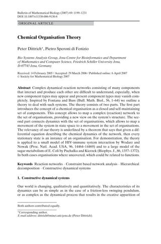
  • 4. 1202 Dittrich and di Fenizio considering a state, e.g. a concentration vector, we limit ourself to the analysis of the set of molecules present in that state. 2.1. Algebraic chemistry We introduce the concept of an algebraic chemistry, which effectively is the re- action network (including stoichiometric information), but that neglects the dy- namics (kinetic laws). The algebraic chemistry represents the required input data structure, from which we will derive the organisational structure of the reaction system. In this work we will refer often to multisets. A multiset is a collection of ob- jects such that each object can appear with a multiplicity higher than 1. As such a multiset is essentially a set where the same object can appear more than one time. Generally the frequency of occurrence of an element a in a multiset A is denoted by #(a ∈ A). Also given a set C we will also refer to PM (C) as the set of all multisets with elements from C. Definition 1 (algebraic chemistry). Given a set M of elements, called molecules, and a set of reaction rules R given by the relation R : PM (M) × PM (M). We call the pair M, R an algebraic chemistry. For simplicity, we adopt the notation from chemistry to write reaction rules. In- stead of writing ({s1 , s2 , . . . , sn }, {s1 , s2 , . . . , sn }) ∈ R we write: s1 + s2 + · · · + sn → s1 + s2 + · · · + sn . Given the left hand side molecules A = {s1 , s2 , . . . , sn } and the right hand side molecules B = {s1 , s2 , . . . , sn }, we write (A → B) ∈ R instead of (A, B) ∈ R. A → B represents a chemical reaction equation where A is the multi- set of molecules on the left hand side (also called reactants) and B the multiset of molecules on the right hand side (also called products). 2.1.1. Input and output There are many processes that give rise to an inflow and outflow, such as, incident sunlight, decaying molecules, or a general dilution flow. In this paper we interpret the reaction rule ∅ → a as an input of a, and a → ∅ as an output of a (∅ denoting the empty set). In the example that follows (Fig. 1) b, c and d decay spontaneously. Example 2. (algebraic chemistry). In this paper we will illustrate the new con- cepts using a small example where there are just four molecular species M = {a, b, c, d}, which react according to the following reaction rules R = {a + b → a + 2b, a + d → a + 2d, b + c → 2c, c → b, b + d → c, b → ∅, c → ∅, d → ∅}. A graphical representation of this reaction network can be found in Fig. 1. 2.2. Semi-organisation:= closed and semi-self-maintaining set In classical analysis, we study the movement of the system in state space. Instead, here, we consider the movement from one set of molecules to another. As in the
  • 5. Chemical Organisation Theory 1203 Fig. 1 Example with four species. Reaction network (a ‘2’ means that two molecules are pro- duced) and graphical representation of the lattice of all sets. The vertical position is determined by the set size. The solid lines depict the lattice of organisations. classical analysis of the dynamics of the system, where fixed points and attractors are considered more important than other states, some sets of molecules are more important than others. In order to find those sets, we introduce some properties that define them, namely: closure, semi-self-maintenance, semi-organisation, self- maintenance, and finally being an organisation. All definitions herein refer to an algebraic chemistry M, R . 2.2.1. Closed sets The first requirement, called closure, assures that a no new molecule can be gen- erated by the reactions inside a set or equivalently that all molecules that can be generated by reactions inside a set are already inside the set Definition 3 (closed set). A set C ⊆ M is closed, if for all reactions (A → B) ∈ R, with A a multiset of elements in C (A ∈ PM (C)), then B is also a multiset of elements in C (B ∈ PM (C)). Given a set S ⊆ M, we can always generate its closure GCL (S) according to the following definition: Definition 4 (generate closed set). Given a set of molecules S ⊆ M, we define GCL (S) as the smallest closed set C containing S. We say that S generates the closed set C = GCL (S) and we call C the closure of S.
  • 6. 1204 Dittrich and di Fenizio We need to prove that this definition is unambiguous: Let us suppose, ad absurdum, that we can find two smaller closed sets U, V with S ⊆ U, V and U = V. Since the intersection of closed sets is trivially closed, so U ∩ V would be closed too but S ⊆ U ∩ V. Thus, we have found a closed set smaller than U and V that contains S, against the supposition. Example 5 (closed sets). In our example test bed (Example 2) there are 10 closed sets: {}, {a}, {b}, {d}, {a, b}, {b, c}, {a, d}, {a, b, c}, {b, c, d} and {a, b, c, d}. The empty set is closed, because there is no input. If there would be an input, the smallest closed set would be the closed set generated from the input set. Assume, for exam- ple, that the reaction rule ∅ → c is added to the set of reaction rules R. In order to find the closed set generated by the input set {c}, we have to add all reaction products among molecules of that set and insert them into that set, until no new molecule can be inserted anymore (for infinite systems, a limit has to be taken). So, the smallest closed set would be {c, b}, and there would be a total number of 4 closed sets left, namely: {b, c}, {a, b, c}, {b, c, d} and {a, b, c, d}. A common algebraic concept that we shall use very often, from now on, is the lattice. A lattice, is a partially ordered set (poset) in which any two elements have a greatest lower bound and a least upper bound (see Supplement or Wikipedia, 2004). Given the generate closed set operator we can trivially define two basic opera- tions, a union operation (U CL V) and an intersection operation (U CL V): U CL V ≡ GCL (U ∪ V), and (1) U CL V ≡ GCL (U ∩ V). (2) Trivially, closed sets, with the operations CL and CL , form a lattice OCL , CL , CL . Closure is important because the closed set generated by a set (its closure) rep- resents the largest possible set that can be reached from a given set of molecules. Furthermore a set that is closed cannot generate new molecules and is in that sense more stable with respect to novelty. As such the concept of closure alone can al- ready give valuable insigh into the structure and organisation of complex chemical ¨ networks as shown by Ebenhoh et al. (2004). 2.2.2. Semi-self-maintaining sets The next property, called semi-self-maintenance, assures that every molecule that is consumed within a set, is produced within that set. We say that a molecule k ∈ M is produced within a set C ⊆ M, if there exists a reaction (A → B), with both A, B ∈ PM (C), and #(k ∈ A) < #(k ∈ B). In the same way, we say that a molecule k ∈ C is consumed within the set C, if, there is a reac- tion (A → B) with A, B ∈ PM (C), and #(k ∈ A) > #(k ∈ B). Definition 6 (semi-self-maintaining set). A set of molecules S ⊆ M is called semi- self-maintaining, if all molecules s ∈ S that are consumed within S are also pro- duced within that set S.
  • 7. Chemical Organisation Theory 1205 Example 7 (semi-self-maintaining sets). In our example system (Example 2) there are 8 semi-self-maintaining sets: {}, {a}, {a, b}, {b, c}, {a, d}, {a, b, c}, {a, b, d}, and {a, b, c, d}. Note that the concept of (semi-) self-maintenance is closely related to the con- ¨ cept of an autocatalytic set (Rossler, 1971; Eigen, 1971; Kauffman, 1971). An au- tocatalytic set is usually defined as a set of molecules such that each molecule is produced by at least one catalytic reaction within that set, see e.g. Ref. Jain and Krishna (2001). 2.2.3. Semi-organisations Taking closure and semi-self-maintenance together, we arrive at the concept of semi-organisation. Definition 8. (semi-organisation). A semi-organisation O ⊆ M is a set of molecules that is closed and semi-self-maintaining. Example 9. (semi-organisation). In our example system (Example 2) except {a, b, d}, all semi-self-maintaining sets are closed, so there are 7 semi-organisations: {}, {a}, {a, b}, {b, c}, {a, d}, {a, b, c} and {a, b, c, d}. 2.3. Organisation:= closed and self-maintaining set In a semi-organisation, all molecules that are consumed are produced; yet this does not guarantee that the total amount of mass can be maintained. A simple coun- terexample is the following reversible reaction in a flow reactor: M = {a, b}, R = {a → b, b → a, a → ∅, b → ∅}. Both molecules, a and b, decay. O = {a, b} is a semi-organisation, because the set is closed, a is produced by the reaction b → a, and b is produced by the reaction a → b. But, obviously, the system {a, b} is not stable, in the sense that there is no stable state in which the two molecules a and b have positive concentrations: both molecules decay and cannot be sufficiently reproduced, and thus they will finally vanish. The solution to this problem is to consider the overall ability of a set to maintain its total mass. We call such sets simply self-maintaining. 2.3.1. Self-maintaining sets Definition 10 (self-maintaining). Given an algebraic chemistry M, R with m = |M| molecules and n = |R| reactions, and let S = (si, j ) be the (m × n) stoichiometric matrix implied by the reaction rules R, where si, j denotes the num- ber of molecules of type i produced in reaction j. A set of molecules C ⊆ M is called self-maintaining, if there exists a flux vector v ∈ Rn such that the follow- ing three conditions apply: (1) for all reactions (A → B) with A ∈ PM (C) the flux v(A→B) > 0; (2) for all reactions (A → B) with A ∈ PM (C), v(A→B) = 0; and (3) for / all molecules i ∈ C, the production rate fi = (Sv)i ≥ 0 with ( f1 , . . . , fm)T = Sv.
  • 8. 1206 Dittrich and di Fenizio v(A→B) denotes the element of v describing the flux (i.e. rate) of reaction A → B. fi is the production rate of molecule i given flux vector v. It is practically the sum of fluxes producing i minus the fluxes consuming i. For the example above, the stoichiometric matrix becomes S = ((−1, 1), (1, −1), (−1, 0), (0, −1)), and we can see that there is no positive flux vector v ∈ R4 , such that Sv ≥ 0. In fact, in that example, only the empty semi-organisation {} is self-maintaining. In case a and b would not decay, R = {a → b, b → a}, the set {a, b} would be (as desired) self- maintaining, because there is a flux vector, e.g., v = (1.0, 1.0), such that Sv = 0 ≥ 0 with S = ((−1, 1), (1, −1)). Example 11 (self-maintaining). In our example system (Example 2) all semi- self-maintaining sets, except {b, c}, are also self-maintaining, so there are 7 self-maintaining sets: {}, {a}, {a, b}, {a, d}, {a, b, c}, {a, b, d}, and {a, b, c, d}. The criterion for self-maintenance will be illustrated by looking at the self- maintaining set S = {a, b} in more detail. Let us first look at the stoichiometric matrix: ⎛ ⎞ 0 0 0 0 0 0 0 0 ⎜1 −1 −1 −1 0 ⎟ ⎜ 0 1 0 ⎟ S=⎜ ⎜0 ⎟. (3) ⎝ 0 1 −1 1 0 −1 0 ⎟ ⎠ 0 1 0 0 −1 0 0 −1 Each column represents a reaction, and each row one molecular species. A positive number implies that the molecule gets produced by the reaction while a negative that the molecule gets consumed by the reaction. Now we have to find all the re- actions active within S, this means to find all reactions (A → B) ∈ R where the lefthand side A is a multiset from S (A ∈ PM (S)). There are two such reactions in the system: a + b → a + 2b and b → ∅. These reactions correspond to column 1 and column 6 of the matrix S and to the fluxes v1 = v(a+b→a+2b) and v6 = v(b→∅) , re- spectively. According to the definition of self-maintenance, these two fluxes must be positive while the remaining fluxes must be zero. Now, in order to show that S = {a, b} is self-maintaining, we have to find positive values for v1 and v6 such that a and b are produced at a non-negative rate. Here, this can be achieved by setting v1 = v6 = 1. So that the flux vector v becomes: ⎛ ⎞ ⎛ ⎞ v1 1 ⎜ v2 ⎟ ⎜ 0 ⎟ ⎜ ⎟ ⎜ ⎟ ⎜v ⎟ ⎜0⎟ ⎜ 3⎟ ⎜ ⎟ ⎜v ⎟ ⎜0⎟ ⎜ 4⎟ ⎜ ⎟ v=⎜ ⎟=⎜ ⎟ (4) ⎜ v5 ⎟ ⎜ 0 ⎟ ⎜ ⎟ ⎜ ⎟ ⎜ v6 ⎟ ⎜ 1 ⎟ ⎜ ⎟ ⎜ ⎟ ⎝ v7 ⎠ ⎝ 0 ⎠ v8 0
  • 9. Chemical Organisation Theory 1207 and ⎛ ⎞ 1 ⎜0⎟ ⎜ ⎟ ⎛ ⎞⎜ ⎟ ⎛ ⎞ ⎛ ⎞ 0 0 0 0 0 0 0 0 ⎜0⎟ 0 f1 ⎜ ⎟ ⎜ ⎟⎜ ⎟ ⎜ ⎟ ⎜ ⎟ ⎜1 0 −1 1 −1 −1 0 0 ⎟⎜0⎟ ⎜0⎟ ⎜ f2 ⎟ Sv = ⎜ ⎟⎜ ⎟ = ⎜ ⎟ = ⎜ ⎟. (5) ⎜0 ⎝ 0 1 −1 1 0 −1 0 ⎟⎜0⎟ ⎜0⎟ ⎜ ⎠⎜ ⎟ ⎝ ⎠ ⎝ f3 ⎟ ⎠ ⎜ ⎟ 0 1 0 0 −1 0 0 −1 ⎜ 1 ⎟ 0 f4 ⎜ ⎟ ⎜0⎟ ⎝ ⎠ 0 As we can see, both molecules are produced at a non-negative rate ( f1 ≥ 0) and ( f2 ≥ 0). So, we can conclude that {a, b} is self-maintaining. Note that we can also chose v1 and v6 such that b is produced at a positive rate ( f2 > 0), e.g., for v1 = 2 and v6 = 1 we get f2 = 1. Note further that, in Example 1, molecule a will always be produced at zero rate ( f1 = 0), independently on how we chose v. Lemma 12. Every self-maintaining set is semi-self-maintaining. Proof: Given a self-maintaining set S ⊆ M, we have to show that every molecule that is consumed by a reaction within the set S is produced by a reaction within that set. Formally, we have to show that for all k ∈ S, if there is a reaction (A → B) ∈ R with A ∈ PM (S), and #(k ∈ A) > #(k ∈ B), then there is also reaction (A → B) ∈ R with A ∈ PM (S) and #(k ∈ A) < #(k ∈ B). So, we have only to care for the molecules k that are consumed: molecules that are consumed have a negative entry in the stoichiometric matrix. Since we demand for a self-maintaining set that their net production is non-negative there must be at least one additional positive entry, which represents a reaction rule in which k is produced. Note that the empty set is always self-maintaining (as it has nothing to maintain) and the set of all possible molecules is always closed (as there is nothing that can be added to it). On the other hand the empty set is not necessarily closed, and the set of all possible molecules is not necessarily self-maintaining. 2.3.2. Organisations Together, closure and self-maintenance together lead to the central definition of this work1 : Definition 13 (organisation). A set of molecules O ⊆ M that is both closed and self-maintaining is called an organisation. 1 Note that our definition of an organisation reads like the definition by Fontana and Buss (1994), however we are using a more general definition of self-maintenance.
  • 10. 1208 Dittrich and di Fenizio An organisation represents an important combination of molecular species, which are likely to be observed in a large reaction vessel on the long run. A set of molecules that is not closed or not self-maintaining would not exists for a long time, because new molecules will appear and others will vanish, respectively. From Lemma 12 trivially follows that: Lemma 14. Every organisation is a semi-organisation. Example 15 (four species reaction system). In our example (Example 2) there are 9 closed sets, 8 semi-self-maintaining sets, 7 self-maintaining sets, and 7 semi- organisations, 6 of which are organisations. Although the reaction system is small, its organisational structure is already difficult to see when looking at the rules or their graphical representation (Fig. 1). In Fig. 1, all 16 possible sets of molecules are shown as a lattice. Finding all organisations of a general reaction system appears to be computa- tionally difficult (Section 5.2). One approach is to find the semi-organisations first, and then check, which of them are also self-maintaining. 2.4. Consistent reaction systems The property of the set of organisations and semi-organisations depends strongly on the type of system studied. In this section we discuss a class of systems, called consistent reaction systems, where given any set we can “nicely” generate an orga- nization and where the set of organisations always forms an algebraic lattice. We will gradually build the definition of a consistent system by presenting some useful intermediate concepts: Definition 16 (semi-consistent). An algebraic chemistry M, R is called semi- consistent, if given any two sets A and B, both semi-self-maintaining, then their union A∪ B is still semi-self-maintaining; and given any two sets A and B, both self-maintaining, then their union A∪ B is still self-maintaining. This definition trivially implies that given any set C there always exists a biggest (semi-)self-maintaining set contained in C. Note also that because in general sys- tems the intersection of closed sets is closed, then also for every set C, there is a smallest closed set containing C. We now start to define three basic operators: generate closure, generate semi- self-maintenance, and generate self-maintenance. Definition 17 (generate semi-self-maintaining set). Given a semi-consistent alge- braic chemistry, on a set M, and given a set of molecules C ⊆ M, we define GSSM (C) as the biggest semi-self-maintaining set S contained in C. We say that C generates the semi-self-maintaining set S = GSSM (C). Definition 18 (generate self-maintaining set). Given a semi-consistent algebraic chemistry, on a set M, and given a set of molecules C ⊆ M, we define GSM (C)
  • 11. Chemical Organisation Theory 1209 as the biggest self-maintaining set S contained in C. We say that C generates the self-maintaining set S = GSM (C). For semi-consistent reaction systems, GSM (C) is always defined, because the union (∪) of two self-maintaining sets is self-maintaining; and further, every set is either self-maintaining, or it contains a unique biggest self-maintaining set. Thus from every set we can generate a self-maintaining set. As usual, the union SM and in- tersection SM of self-maintaining sets S1 , S2 are defined as S1 SM S2 ≡ GSM (S1 ∪ S2 ) = S1 ∪ S2 , S1 SM S2 ≡ GSM (S1 ∩ S2 ), respectively. Thus also the set of all self- maintaining sets OSM , in a semi-consistent system, forms a lattice OSM , SM , SM . Equivalently we can generate the lattice of semi-self-maintaining sets. Note that we make no requirement that the largest semi-self-maintaining set in C be itself self-maintaining. In other words we do not require that the largest semi-self-maintaining set and the largest self-maintaining set be the same. Lemma 19. In semi-consistent systems the following statements are equivalent: the closure of a (semi-)self-maintaining set is (semi-)self-maintaining and the (semi-) self-maintaining set generated by a closed set is closed. Proof: Let us suppose that the first statement is true, we shall prove the second: Let C be a closed set. Let S = GSM (C) be the self-maintaining set generated by C. Let D be the closure of S. Then D ⊆ C, because the closure of S cannot pro- duce any molecule not contained in the closed set C. So S ⊆ D ⊆ C. But D is self-maintaining (because the closure of a self-maintaining set is closed). Yet S by construction is the biggest self-maintaining set in C. Thus S = D. So S is closed. Let us now suppose that the second statement is true, we shall prove the first: Let S be a self-maintaining set. Let C = GCL (S) be the closure of S. Let D be the self-maintaining set generated by C. Then S ⊆ D, because D is the biggest self- maintaining set, and if not we could take the union between S and D, which would still be a self-maintaining set, bigger than D. Since the self-maintaining set gener- ated by a closed set is closed, then D is closed. So D is closed and self-maintaining. But since C is the closure of S, then C has to be the smallest closed set containing S. Thus C ⊆ D. So C = D. Thus C is closed and then the closure of S must return the smallest closed set that contains S. So C must be self-maintaining. Definition 20 (consistent). A semi-consistent algebraic chemistry is called consis- tent if the closure of a semi-self-maintaining set is semi-self-maintaining and the closure of a self-maintaining set is self-maintaining. With Lemma 19 this implies also that the (semi-)self-maintaining set generated by a closed set is also closed. Trivially, the self-maintaining set generated by a semi- self-maintaining set is semi-self-maintaining and the semi-self-maintaining set gen- erated by a self-maintaining set is the set itself, thus is self-maintaining. In other words consistent reaction systems are systems where the three gener- ate operators behave nicely one respect to the other: each operator can be used after any other, and the acquired properties are not lost when the new operator
  • 12. 1210 Dittrich and di Fenizio is applied. This gives us the possibility to define the (semi-)organisation generated by a set. There are many ways in which we can generate a semi-organisation from a set. We will present here the simplest one, which implicitly assumes that molecules are produced quickly and vanish slowly. This assumption leads to the largest possible semi-organisation generated by a set: Definition 21 (generate semi-organisation). Given a consistent algebraic chem- istry and a set of molecules C ⊆ M, we define GSO (C) as GSSM (GCL (C)). We say that C generates the semi-organisation O = GSO (C). Finally, in consistent reaction systems, we can also generate uniquely an organ- isation, (here, again, the largest organisation that can be generated from a set) according to the following definition: Definition 22 (generate organisation). Given a set of molecules C ⊆ M, we define G(C) as GSM (GCL (C)). We say that C generates the organisation O = G(C). The following lemma summarises the situation for consistent reaction systems: Lemma 23. In a consistent reaction system, given a set C, we can always uniquely generate a closure GCL (C), a semi-self-maintaining set GSSM (C), a semi- organisation GSSM (GCL (C)), a self-maintaining set GSM (C), and an organisation GSM (GCL (C)). Following the same scheme as before, the union ( SO ) O and intersection ( SO ) O of two (semi-)organisations U and V is defined as the (semi-)organisation generated by their set-union and set-intersection: (U SO V ≡ GSO (U ∪ V), U SO V ≡ GSO (U ∩ V)), U O V ≡ G(U ∪ V), U O V ≡ G(U ∩ V), respectively. Thus, for consistent reaction systems, also the set of all (semi-)organisations (OSO ) O forms a lattice ( OSO , SO , SO ) O, O , O . This important fact should be em- phasised by the following lemma: Lemma 24. Given an algebraic chemistry M, R of a consistent reaction system and all its organisations O, then O, O , O is a lattice. Knowing that the semi-organisations and organisations form a lattice, and that we can uniquely generate an organisation for every set, is a useful information. In order to find the whole set of organisations, it is impractical just to check all the possible sets of molecules. Instead, we can start by computing the lattice of semi- organisations, and then test only those sets for self-maintenance. Furthermore, if the semi-organisations form a lattice, we can start with small sets of molecules and generate their semi-organisations, while the SO operator can lead us to the more complex semi-organisations. Now we will present three types of consistent systems, which can be easily (i.e. in linear time) identified by looking at the reaction rules.
  • 13. Chemical Organisation Theory 1211 2.4.1. Catalytic flow system In a catalytic flow system all molecules are consumed by first-order reactions of the form {k} → ∅ (dilution) and there is no molecule consumed by any other reaction. So, each molecule k decays spontaneously, or equivalently, is removed by a dilu- tion flow. Apart from this, each molecule can appear only as a catalyst (without being consumed). Definition 25 (catalytic flow system). An algebraic chemistry M, R is called a catalytic flow system, if for all molecules i ∈ M: (1) there exists a reaction ({i} → ∅) ∈ R, and (2) there does not exist a reaction (A → B) ∈ R with (A → B) = ({i} → ∅) and #(i ∈ A) > #(i ∈ B). Examples of catalytic flow system are the replicator equation (Schuster and Sigmund, 1983), the hypercycle (Eigen, 1971; Eigen and Schuster, 1977), the more general catalytic network equation (Stadler et al., 1993), or AlChemy (Fontana, 1992). Furthermore some models of genetic regulatory networks and social system (Dittrich et al., 2003) are catalytic flow systems. The proof that a catalytic flow system is a consistent reaction system will be given later as part of the more general proof that the more general reactive flow system with persistent molecules is a consistent reaction system (Lemma 32). Example 26 (catalytic flow system). As an example, we present a three-membered elementary hypercycle (Eigen, 1971; Eigen and Schuster, 1977) under flow condi- tion. The set of molecules is defined as: M = {a, b, c} (6) and the reaction rules as: R={ (7) a + b → a + 2b, (8) b + c → b + 2c, (9) c + a → c + 2a, (10) a → ∅, (11) b → ∅, (12) c→∅ (13) }. (14) We can see, that all three molecules decay by first-order reactions (representing the dilution flow), and that no molecule is consumed by any of the three remaining reactions.
  • 14. 1212 Dittrich and di Fenizio Lemma 27. In a catalytic flow system, all semi-self-maintaining sets are self- maintaining. Proof: We proof the lemma by constructing a flux vector v = (v1 , . . . , vn ), n = |R|, that follows the self-maintaining conditions. From the definition note that in a cat- alytic flow system all molecules are consumed by first-order reactions of the form {k} → ∅ and there is no molecule consumed by any other reaction. Also from the definition of a catalytic flow system we know that all molecules decay. Given a semi-self-maintaining set S ⊆ M we construct v as follows: (i) set all fluxes for reactions among molecules that are not a subset of S to 0: v(A→B) = 0 for (A → B) ∈ R, A ∈ PM (S). / (ii) Since all molecules decay we set all fluxes of molecules from S that correspond to decay reactions to 1: ∀i ∈ S,v({i}→∅) = 1. (iii) Because S is semi-self-maintaining, there must be for each i ∈ S one or more reactions of the form (A → B) ∈ R, A ∈ PM (S) where i is produced. We set the flux of those reactions to v(A→B) > 1. Since all reactions are purely catalytic, no molecule is consumed by (iii). On the other hand each molecule in S is generated by (iii) with a flow greater than the dilution flow. Thus we found a flow that meets the conditions of a self-maintaining set, thus S is self-maintaining. Note that, as before, when writing v(A→B) we use the reaction A → B as an index in order to refer to the flux vector’s element corresponding to this reaction. Lemma 28. In a catalytic flow system, every semi-organisation is an organisation. Proof: Follows immediately from Lemma 27. In a catalytic flow system we can easily check, whether a set O is an organisation by just checking whether it is closed and whether each molecule in that set is produced by that set. Furthermore, given a set A, we can always generate an organisation by adding all molecules produced by Auntil Ais closed and then removing molecules that are not produced until A is semi-self-maintaining. With respect to the inter- section and union of (semi-)organisations the set of all (semi-) organisations of a catalytic flow system forms an algebraic lattice (see below). A result which has already been noted by Fontana and Buss (1994). 2.4.2. Reactive flow system In a reactive flow system all molecules are consumed by first-order reactions of the form {k} → ∅ (dilution). But in addition to the previous system, we allow arbitrary additional reactions in R. Thus note how a catalytic flow system is a particular kind of reactive flow system. Definition 29 (reactive flow system). An algebraic chemistry M, R is called a re- active flow system, if for all molecules i ∈ M, there exists a reaction ({i} → ∅) ∈ R.
  • 15. Chemical Organisation Theory 1213 This is a typical situation for chemical flow reactors or bacteria that grow and di- vide (Puchalka and Kierzek, 2004). In a reactive flow system, semi-organisations are not necessarily organisations. Nevertheless, both the semi-organisations and the organisations form a lattice O, O , O . Moreover, the union ( O ) and inter- section ( O ) of any two organisations is an organisation. Also the proof that a reactive flow system is a consistent reaction system will be given later as part of the same general proof that the more general reactive flow system with persistent molecules is a consistent reaction system (Lemma 32). Example 30 (reactive flow system). As an example, we take the three-membered elementary hypercycle as before, but add an explicit substrate s. The set of molecules is defined as: M = {a, b, c, s} (15) and the reaction rules as: R={ (16) a + b + s → a + 2b, (17) b + c + s → b + 2c, (18) c + a + s → c + 2a, (19) a → ∅, (20) b → ∅, (21) c → ∅, (22) s→∅ (23) }. (24) We can see that again all molecules decay by first-order reactions (represent- ing the dilution flow), but now a molecule, s, is consumed by other reactions (Eq. 17–19). Note that in this example there is only one organisation (the empty or- ganisation), and even no semi-organisation that contains one or more molecules, because there is no inflow of the substrate. If we would add a reaction equation ∅ → s representing an inflow of the substrate, we would obtain two organisations: {s} and the “hypercycle” {a, b, c, s}. 2.4.3. Reactive flow system with persistent molecules In a reactive flow system with persistent molecules there are two types of molecules: persistent molecules P and non-persistent molecules. All non-persistent molecules k ∈ M P are consumed (as in the two systems before) by first-order reactions of
  • 16. 1214 Dittrich and di Fenizio the form {k} → ∅; whereas a persistent molecule p ∈ P is not consumed by any reaction at all. Definition 31 (reactive flow system with persistent molecules). An algebraic chem- istry M, R is called a reactive flow system with persistent molecules, if we can partition the set of molecules in persistent P and non-persistent molecules P ¯ (M = P ∪ P, P ∩ P = ∅) such that: (i) for all non-persistent molecules i ∈ P: ¯ ¯ ¯ there exists a reaction ({i} → ∅) ∈ R; and (ii) for all persistent molecules i ∈ P: there does not exist a reaction (A → B) ∈ R with #(i ∈ A) > #(i ∈ B). An example of a reactive flow system with persistent molecules is Example 2, where a is a persistent molecule. The reactive flow system with persistent molecules is the most general of the three systems where the semi-organisations and organisations always form a lattice, and where the generate organisation operator can be prop- erly defined. As in a reactive flow system, in a reactive flow system with persistent molecules not all semi-organisations are organisations. The previously mentioned fact that reactive flow system with persistent molecules, reactive flow system and catalytic flow system are consistent will be now formulated as a proposition and proven by Lemmas 33–38. Since a catalytic flow system is a particular kind of reactive flow system, and a reactive flow system is a particular kind of reactive flow system with persistent molecules, it is sufficient to consider a reactive flow system with persistent molecules. Proposition 32. A reactive flow system with persistent molecules is consistent. Proof: We need to show that: (1) given any couple of (semi-)self-maintaining sets, their union is (semi-)self-maintaining (thus is a semi-consistent system); (2) given a (semi-)self-maintaining set the closure of it is (semi-)self-maintaining. We shall also prove, although not strictly necessary that (3) given a closed set the (semi-) self-maintenance generated by it, is closed. Lemma 33. In a reactive flow system with persistent molecules, given two semi- self-maintaining sets, A, B ⊆ M, their set-union A∪ B is semi-self-maintaining. Proof: In a reactive flow system with persistent molecules there are two types of molecules: persistent molecules P and non-persistent molecules. We need to prove that there are production pathways for each non persistent molecule. From the definition we know that all non-persistent molecules k ∈ M P of a reactive flow system with persistent molecules are used-up by first-order reactions of the form {k} → ∅ (meaning that they decay spontaneously). Because A and B are self- maintaining, there must be a production pathway of these molecules already inside A or B. Thus A∪ B is semi-self-maintaining. Lemma 34. In a reactive flow system with persistent molecules, given two self- maintaining sets, A, B ⊆ M, their set-union A∪ B is self-maintaining.
  • 17. Chemical Organisation Theory 1215 Proof: In a reactive flow system with persistent molecules there are two types of molecules: persistent molecules P and non-persistent molecules. A persistent molecule p ∈ P is not used-up by any reaction of R. So, a persistent molecule can- not have a negative production rate in any set. From the definition we know that all non-persistent molecules k ∈ M P of a reactive flow system with persistent molecules are used-up by first-order reactions of the form {k} → ∅ (meaning that they decay spontaneously). Because Aand B are self-maintaining, there must be a positive production of these molecules in order to compensate their decay. In the union of A and B there might be additional reactions that use up non-persistent molecules, but since there are pathways in A or B to produce them in arbitrary quantity (note that the definition of self-maintenance requires only that there ex- ists a flux vector), we can still find a flux vector such that they are produced at a non-negative total rate. Lemma 35. In a reactive flow system with persistent molecules, given a closed set the semi-self-maintaining set generated by it, is closed. Proof: Let C be a closed set and S = GSSM the semi-self-maintaining set gener- ated by C. Let us assume ad absurdum that S is not closed. Then we can find a molecule a ∈ S that can be produced by S. If S ∪ {a} is semi-self-maintaining, then / we have a set that is bigger than S and semi-self-maintaining, against the definition of S as the biggest semi-self-maintaining set in C. If instead S ∪ {a} is not semi- self-maintaining, then there exist a molecule in S ∪ {a} that is not being generated. This molecule cannot be a, because a is generated by S. So this molecule would have to be b ∈ S. If b is persistent, then it does not need to be generated. If b is not persistent, then there is an outflow that destroys b, thus b must have been gener- ated from within S. So b is still being generated in S ∪ {a}. So, also this possibility is excluded. Thus the set S has to be closed. Lemma 36. In a reactive flow system with persistent molecules, given a semi-self- maintaining set the closure of it is semi-self-maintaining. Proof: Follows directly from the previous Lemma 35 and Lemma 19, which we can apply because Lemma 33 and Lemma 34 assures that a reactive flow system with persistent molecules is semi-consistent. Lemma 37. In a reactive flow system with persistent molecules, given a self- maintaining set the closure of it is self-maintaining. Proof by induction: Let S be a self-maintaining set and C = GCL (S) = S ∪ C1 ∪ C2 ∪ . . . its closure, where C1 contains all molecules from S and the molecules that can be generated directly by S. Ci+1 i contains all molecules from Ci and the molecules that can be generated directly by Ci . Now, let us suppose that Ci is self- maintaining. Then there exist a flux vector v for Ci fulfilling the self-maintenance condition. Let us consider all molecules in Ci+1 Ci . Each of those molecules is produced by the flux vector v at a non negative rate. So we need now to find a flux vector v for Ci+1 . Let us start by taking the same flux vector v we had for the
  • 18. 1216 Dittrich and di Fenizio molecules of Ci . We can produce the non persistent molecules in Ci at an arbitrary large rate. In fact we can consider the molecule that is generated the least as being overproduced at a rate of 1. Each of the new molecules can also be generated at a rate bigger or equal than 1 by the reactions in Ci . Now we need to build the flux v , but v is equal to v for each reaction among molecules that are contained in Ci . Let us consider that we have n new reactions, with m being the maximum stoichiomet- ric coefficient of those reactions, we can then define the speed of the new reactions as 1/m(n + 1), guaranteeing that every molecule in Ci+1 is produced at a positive rate. Thus Ci+1 is self-maintaining. Lemma 38. In a reactive flow system with persistent molecules, given a closed set the self-maintaining set generated by it is closed. Proof: Follows directly from the previous Lemma 37 and Lemma 19, which we can apply because Lemma 33 and Lemma 34 assures that a reactive flow system with persistent molecules is semi-consistent. And this concludes the proof that a reactive flow system with persistent molecules is consistent. As a summary, from a practical point of view, we can first calculate the set of semi- organisations. If our system is a catalytic flow system , we automatically obtain the lattice of organisations. Otherwise we have to check for each semi-organisation whether it is self-maintaining or not. If we have a consistent reaction system, then we are assured to obtain a lattice, where there is a unique smallest and largest organisation, and where we can easily obtain the intersection and union of two organisations from the graphical representation of the lattice (see examples). For a general reaction system, the set of organisations does not necessarily form a lattice. Nevertheless, this set of organisations represent the organisational structure of the reaction network, which can be visualised and which can provide a new view on the dynamics of the system by mapping the movement of the system in state space to a movement in the set of organisations, as will be shown in Section 3. 2.5. General reaction systems When we consider general reaction systems, i.e. algebraic chemistries without any constraints, we cannot always generate a self-maintaining set uniquely. This im- plies that in a general reaction system neither the set of organisation nor the set of semi-organisations necessarily form a lattice. Examples of this can be found in planetary atmosphere chemistries (Yung and DeMore, 1999). Example 39 (General reaction system without a lattice of organisation). In this example we present a reaction system where the set of organisations does not form a lattice, and where we can not always generate an organisation for any given set of molecules: M = {a, b, c}, R = {a + b → c}. (25) This example can be interpreted as an isolated system, where there is no inflow nor outflow. a and b simply react to form c. Obviously, every set that does not contain
  • 19. Chemical Organisation Theory 1217 Fig. 2 Example of a general reaction system that does not have a lattice of organisations. There are three molecules M = {a, b, c} and just one reaction rule R = {a + b → c}. a together with b is an organisation. So, there are 6 organisations: {}, {a}, {b}, {c}, {a, c}, and {b, c}. As illustrated by Fig. 2, there is no unique largest organisation and therefore the set of organisations does not form a lattice. Furthermore, given the set {a, b, c}, we cannot generate an organisation uniquely, because there does not exist a unique largest self-maintaining set contained in {a, b, c}. There are two self-maintaining sets of equal size: {a, c} and {b, c}. Why can this not happen in a reactive flow system with persistent molecules? In a reactive flow system with persis- tent molecules, the set-union of two self-maintaining sets is again self-maintaining. Therefore there can not exist two largest self-maintaining sets within a set A, be- cause their union would be a larger self-maintaining set within A(see Lemma 34). Note that each organisation makes sense, because each organisation represents a combination of molecules that can stably exists in a reaction vessel, which does not allow an outflow of any of the molecules according to the rules R. 3. Dynamic analysis The static theory deals with molecules M and their reaction rules R, but not with the evolution of the system in time. To add dynamics to the theory, we have to formalise the dynamics of a system. In a very general approach, the dynamics is given by a state space X and a formal definition (mathematical or algorithmic) that describes all possible movements in X only. Given an initial state x0 ∈ X, the formal definition describes how the state changes over time. For simplicity, we assume a deterministic dynamical process, which can be formalised by a phase flow (X, (Tt )t∈R ) where (Tt )t∈R is a one-parametric group of transformations from X. Tt (x0 ) denotes the state at time t of a system that has been in state x0 at t = 0. 3.1. Connecting to the static theory A state x ∈ X represents the state of a reaction vessel, which contains molecules from M. In the static part of the theory we consider just the set of molecular species present in the reaction vessel, but not their concentrations, spatial distri- butions, velocities, and so on. Now, given the state x of the reaction vessel, we need a function that maps uniquely this state to the set of molecules present. Vice versa, given a set of
  • 20. 1218 Dittrich and di Fenizio molecules A ⊆ M, we need to know, which states from X correspond to this set of molecules. For this reason we introduce a mapping φ called abstraction, from X to P(M), which maps a state of the system to the set of molecules that are present in the system being in that state. The exact mapping can be defined precisely later, depending on the state space, on the dynamics, and on the actual application. The concept of instance is the opposite of the concept of abstraction. While φ(x) denotes the molecules represented by the state x, an instance x of a set Ais a state where exactly the molecules from A are present according to the function φ. Definition 40 (instance of A). We say that a state x ∈ X is an instance of A ⊆ M, iff φ(x) = A. In particular, we can define an instance of an organisation O (if φ(x) = O) and an instance of a generator of O (if G(φ(x)) = O). Loosely speaking we can say that x generates organisation O. Note that a state x of a reactive flow system with persis- tent molecules, reactive flow system, and catalytic flow system is always an instance of a generator of one and only one organisation O. This leads to the important observation that a lattice of organisations partitions the state space X, where a partition XO implied by organisation O is defined as the set of all instance of all generators of O: XO = {x ∈ X|G(φ(x)) = O}. Note that as the system state evolves over time, the organisation G(φ(x(t))) generated by x(t) might change (see below, Figs. 3 and 4). 3.2. Fixed points are instances of organisations Now we will describe a theorem that relates fixed points to organisations, and by doing so, underlines the relevancy of organisations. We will show that, given an ordinary differential equation (ODE) of a form that is commonly used to describe the dynamics of reaction systems, every fixed point of this ODE is an instance (a) (b) 2 2 {b} {a, b} {a} concentration (arbitrary unit) a b 1 [a] (c) a b 0.1 Phi=0.1 a b [b] 0.01 1 10 100 time (arbitrary unit) Fig. 3 Example of an up-movement caused by a constructive perturbation, followed by a down- ward movement. (a) reaction network, (b) concentration vs. time plot of a trajectory, (c) lattice of organisations including trajectory.
  • 21. Chemical Organisation Theory 1219 {a, b, c, d} trajectory down link up link {a, b, c} [a] > 1 [a] <= 1 concentration (arbitrary unit) 1 [a] [b] [a] > 1 {a, b} {a, d} Phi=0.1 0.1 [a] < 1 [a] > 1 [a] > 1 0.01 [d] [c] {a} 0.001 1 10 100 time (arbitrary unit) {} Fig. 4 Lattice of organisations of Example 1, including up-links and down-links. Furthermore a trajectory is shown starting in organisation {a, b, c, d} moving down to organisation {a, b}. of an organisation. We therefore assume in this section that x is a concentration vector x = (x1 , x2 , . . . , x|M| ), X = R|M| , xi ≥ 0 where xi denotes the concentration of molecular species i in the reaction vessel, and M is finite. The dynamics is given by an ODE of the form x = Sv(x) where S is the stoichiometric matrix implied by ˙ the algebraic chemistry M, R (reaction rules). v(x) = (v1 (x), . . . , vn (x)) ∈ R|R| is a flux vector depending on the current concentration x, where |R| denotes the number of reaction rules. A flux v j (x) describes the rate of a particular reaction j. For the function v j we require only that v j (x) is positive, if and only if the molecules on the left hand side of the reaction j are present in the state x, and oth- erwise it must be zero. Often it is also assumed that v j (x) increases monotonously, but this is not required here. Given the dynamical system as x = Sv(x), we can ˙ define the abstraction of a state x formally by using a (small) threshold ≥ 0 such that all fixed points have positive coordinates greater than . Definition 41 (abstraction). Given a dynamical system x = f (x) and let x be a ˙ state in X, then the abstraction φ(x) is defined by φ(x) = {i|xi > , i ∈ M}, φ : X → P(M), ≥0 (26) where xi is the concentration of molecular species i in state x, and is a threshold chosen such that it is smaller than any positive coordinate of any fixed point of x = f (x), xi ≥ 0. ˙ Setting = 0 is a safe choice, because in this case φ always meets the definition above. But for practical reasons, it makes often sense to apply a positive threshold greater zero, e.g., when we take into consideration that the number of molecules in a reaction vessel is finite.
  • 22. 1220 Dittrich and di Fenizio Theorem 42. Hypothesis: Let us consider a general reaction system whose reac- tion network is given by the algebraic chemistry M, R and whose dynamics is given by x = Sv(x) = f (x) as defined before. Let x ∈ X be a fixed point, that is, ˙ f (x ) = 0, and let us consider a mapping φ as given by Def. 41, which assigns a set of molecules to each state x. Thesis: φ(x ) is an organisation. Proof: We need to prove that φ(x ) is closed and self-maintaining: (a) Closure: Let us assume that φ(x ) is not closed, then there exist a molecule k, k ∈ φ(x ), generated by the molecules in φ(x ). Since, x is a fixed point, / f (x ) = Sv(x ) = 0. First we decompose the stoichiometric matrix S into two matrices of the same size of S, S+ and S− , separating all positive from the negative coefficients, respectively, such that S = S+ + S− . Since, by defini- tion, v(x ) is always non-negative, then S+ v(x ) ≥ 0, and S− v(x ) ≤ 0. Let xk ˙+ − + − and xk be the k-th row of S v (x) and S v (x), respectively, which repre- ˙ sent the inflow (production) and outflow (destruction) of molecules of type ˙+ ˙− k. The fixed point condition implies that xk + xk = xk = 0. Since we assumed ˙ ˙+ ˙+ that k is produced by molecules from φ(x ), xk must be positive, xk > 0 and − − thus xk must be negative, xk < 0. But this leads to a contradiction, in fact: ˙ ˙ there are two possible cases: either xk is equal to zero or xk is higher than ˙− zero. If xk = 0, then xk must be zero, too, by definition of flux (intuitively because a molecule not present cannot vanish). If, instead, xk is bigger than zero, still xk must be smaller or equal to our chosen threshold. Or xk would be part of φ(x), against the hypothesis. But we have explicitly chosen to be smaller than every positive coordinate of any fixed point. Thus also this is not possible. (b) Self-Maintenance: We have to show that φ(x ) is self-maintaining. Since x is a fixed point Sv(x ) = 0, which fulfils condition (3) of the definition of self- maintenance (Def. 6). From the requirements for the flux vector v, it follows directly that v(A→B) (x ) > 0 for all A ∈ PM (φ(x )), which fulfils condition (1) of Def. 6. Following the same contradictory argument as before in (ii), xk must be zero for k ∈ φ(x), and therefore v(A→B) (x ) = 0 for A ∈ PM (φ(x)), which fulfils / / the remaining condition (2) of self-maintenance. From this theorem it follows immediately that a fixed point is an instance of a closed set, a semi-self-maintaining set, and of a semi-organisation. Let us finally mention that even if each fixed point is an instance of an organisation, an organisa- tion does not necessarily possess a fixed point. A well known example is exponen- tial growth: M = {a}, R = {a → 2a}, x = Sv(x) with S = 1 and v(x) = x. There are ˙ two organization the empty organization {} and the organization {a}, which repre- sents an exponentially growing population. Obviously there is no fixed point with x > 0. Further note that given an attractor A ⊆ X, there exists an organisation O such that all points of Aare instances of a generator of O. In fact, it might be natural to suppose that all points of an attractor are actually instances of O, yet it is not clear if this is true for all systems or just for some.
  • 23. Chemical Organisation Theory 1221 3.3. Movement from organisation to organisation 3.3.1. ODEs and movement in the set of organisations Not all system can be studied using ODEs. In particular a discrete system is usually only approximated by an ODE. In a discrete dynamical system, the molecular species that are present in the reaction vessel can change in time, e.g, as the last molecule of a certain type vanishes. In an ODE instead, this does not generally happen, where molecules can tend to zero as time tends to infinity. So, even if in reality a molecule disappears, in an ODE model it might still be present in a tiny quantity. The fact that every molecule ends up being present in (at least) a tiny quantity, generally precludes us to notice that the system is actually moving from a state where some molecules are present, to another state where a different set of molecules is present. Yet this is what happens in reality, and in this respect, an ODE is a poor approximation of reality. A common approach to overcome this problem is to introduce a concentration threshold , below which a molecular species is considered not to be present. We use this threshold in order to define the abstraction φ, which just returns the set of molecules present in a certain state. Additionally, we might use the threshold to manipulate the numerical integration of an ODE by setting a concentration to zero, when it falls below the threshold. In this case, a constructive perturbation (i.e. a perturbation that causes a new molecular species to appear) has to be greater than this threshold. 3.3.2. Downward movement Not all organisations are stable. The fact that there exits a flux vector, such that no molecule of that organisation vanishes, does not imply that this flux vector can be realised when taking dynamics into account. As a result a molecular species can disappear. Each molecular species that disappears simplifies the system. Some molecules can be generated back. But eventually the system can move from a state that generates organisation O1 into a state that generates organisation O2 , with O2 always below O1 (O2 ⊂ O1 ). We call this spontaneous movement a downward movement. Figure 4 illustrates this downward movement using the four-species example (Example 2 and Fig. 1). The simulation is performed by numerical integration of an ODE assuming mass-action kinetics. Starting with high concentration of all four molecular species (i.e. starting in organisation {a, b, c, d}) the system moves spontaneously down to organisation {a, b, c} and finally to organisation {a, b}. 3.3.3. Upward movement Moving up to an organisation above requires that a new molecular species appears in the system. This new molecular species cannot be produced by a reaction among present molecules (condition of closure). Thus moving to an organisation above is more complicated then the movement down and requires a couple of specifications that describe how new molecular species enter the system. Here we assume that new molecular species appear by some sort of random perturbations or purposeful interference. We assume that a small quantity of molecules of that new molecular species (or a set of molecular species) suddenly appears. Often, in practice, the
  • 24. 1222 Dittrich and di Fenizio perturbation (appearance of new molecular species) has a much slower time scale than the internal dynamics (e.g., chemical reaction kinetics) of the system. Example 43 (Upward and downward Movement). Assume a system with two molecular species M = {a, b} and the reactions R = {a → 2a, b → 2b, a + b → a, a →, b →}. All combinations of molecules are organisations, thus there are four organisations (Fig. 3). Assume further that the dynamics is governed by the ODE x1 = x1 − x1 , x2 = x2 − x2 − x1 x2 where x1 and x2 denote the concentration ˙ 2 ˙ 2 of species a and b, respectively. We map a state to a set of molecules by using a small, positive threshold = 0.1 > 0 (Def. 41). Now, assume that the system is in state x0 = (0, 1) thus in organisation {b}. If a small quantity of a appears (construc- tive perturbation), the amount of a will grow and b will tend to zero. The system will move upward to organisation {a, b} in a transient phase, while finally moving down and converging to a fixed point in organisation {a}. This movement can now be visualised in the lattice of organisations as shown in Fig. 3. 3.3.4. Visualising possible movements in the set of organisations In order to display potential movements in the lattice or set of organisations, we can draw links between organisations. As exemplified in Figs. 3 and 4, these links can indicate possible downward movements (down-link, blue) or upward move- ments (up-link, red). A neutral link (black line) denotes that neither the system can move spontaneously down, nor can a constructive perturbation move the system up. Whether the latter is true depends on the definition of ‘constructive perturba- tion’ applied. For the example of Fig. 4 we defined a constructive perturbation as inserting a small quantity of one new molecular species. The dynamics in between organisations is more complex than this intuitive pre- sentation might suggest, for example in some cases it is possible to move from one organisation O1 to an organisation O2 , with O2 above (or below) O1 without pass- ing through the organisations in between O1 and O2 . In Fig. 4, this is the case for an upward movement from organisation {a} to organisation {a, b, c} caused by a constructive perturbation where a small quantity of c has been inserted (simula- tion and trajectory not shown). 4. Organisations in real systems In preliminary studies (Speroni di Fenizio et al., 2000) we have shown that artifi- cial chemical reaction networks that are based on a structure-to-function mapping (e.g. Fontana and Buss, 1994; Banzhaf, 1993) possess a more complex lattice of or- ganisation than networks created randomly. From this observation we can already expect that natural networks possess non-trivial organisation structures. Our in- vestigation of planetary photo-chemistries (Yung and DeMore, 1999) and bacte- rial metabolism, revealed lattices of organisations that vanish when the networks are randomised, indicating a non-trivial structure. Here we present three brief examples from our ongoing research. The first ex- ample is a model of HIV-immune system dynamics comprising four species. The simplicity of that model allows us to validate our approach analytically. The second
  • 25. Chemical Organisation Theory 1223 and third example is based on a model of the central sugar metabolism of E. coli by Puchalka and Kierzek (2004) comprising 92 species. It shows that non-trivial network complexity can be tackled and that sub-structures in the model can be identified not known before. 4.1. Example: HIV-immune system dynamics Wodarz and Nowak (1999) developed a model of immunological control of HIV in order to explain the effect of various drug treatment strategies. Especially the model shows, why a specific drug treatment strategy does not try to remove the virus, but aims at stimulating the immune defence, such that the immune system controls the virus at low but positive quantities. In the model, there are four molecular species: M = {x, y, w, z}: uninfected CD4+ T cells x, infected CD4+ T cells y, cytotoxic T Lymphocyte (CTL) precur- sors w, and CTL effectors z. The concentration of each species is specified by x, y, w, and z, respectively. The dynamics is given by an ordinary differential equation (ODE) with kinetic parameters a, b, c, d, h, p, q, β, and λ: x ˙ = λ − dx − βxy, y ˙ = βxy − ay − pyz, (27) w ˙ = cxyw − cqyw − bw, z ˙ = cqyw − hz. From the given deterministic ODE model we derive chemical reaction rules, which form a reaction network (Fig. 5, right top): ∅→ x, x+y→ 2y, x→ ∅, y+z→ z, y→ ∅, R={ x+y+w→ x + y + 2w, w→ ∅, y+w→ y + z, z→ ∅ }. The ODE model includes a decay term for each species. Therefore, for each species, we have a reaction rule transforming that molecular species into the empty set: x → ∅, y → ∅, w → ∅, and z → ∅. We observe in passing that in this particu- lar case, since all species decay, the system is a reactive flow system (Definition 2.4.2), thus consistent (Lemma 32), and therefore the set of organisations must be a lattice (Lemma 24), with one well defined largest and one well defined smallest organisation. A graphical representation of the network is shown in Fig. 5, upper right corner. The corresponding 4 × 9 stoichiometric matrix S reads: ⎛ ⎞ 1 −1 0 0 0 −1 0 0 0 x ⎜ ⎟ y ⎜0 0 −1 0 0 1 −1 0 0 ⎟ S= ⎜ ⎟ w ⎜0 0 0 −1 0 0 0 1 −1 ⎟ ⎝ ⎠ z 0 0 0 0 −1 0 0 0 1
  • 26. 1224 Dittrich and di Fenizio Fig. 5 Illustration of the analysis of the HIV immunological response model by Wodarz and Nowak Wodarz and Nowak (1999). The ODE model given in Eq. (27) is transformed to a chem- ical reaction network (right top). The resulting hierarchy of organisations is shown as a Hasse diagram (right middle). Two of the organisations represent the attractors: virus under control (top organisation) and immune system destruction (middle organisation). Dynamic simulations leading to both attractors are shown on the left. Parameters were taken from Wodarz and Nowak (1999) as follows: λ = 1; d = 0.1; β = 0.5; a = 0.2; p = 1; c = 0.1; b = 0.01; q = 0.5; h = 0.1. Initial concentrations for left, top plot: x = 0.74; y = 0.75; w = 0.018; z = 0.49. Initial concentrations for left, bottom plot: x = 0.75; y = 0.14; w = 0.0095; z = 0.17. At the bottom, the full lattice of sets is shown including closed and self-maintaining sets. where each row corresponds to a molecular species x, y, w, z (from the top) and each column corresponds to a reaction. As we can see, the stoichiometric matrix does not contain all information of the reaction network. For example, the reaction rule y + z → z appears only as the column vector (0, −1, 0, 0)T .
  • 27. Chemical Organisation Theory 1225 4.1.1. Lattice of organisations For applying the theory we check every possible set of species (i.e. 16 sets) whether it is closed and self-maintaining. As a result we found three organisations. The Hasse diagram is depicted in Fig. 5, middle right. The smallest organisation consists only of the ‘healthy cells’ x (uninfected CD4+ T cells). There can not be a smaller organisation (e.g. the empty set), because x is an input species and therefore the empty set is not closed. Since x is an input species, the set {x} is obviously self- maintaining. Looking at the reaction rules we can see that x alone can not produce anything else, thus the set {x} is closed, too. Formally, we can show that {x} is an organisation. The second organisation, {x, y} contains ‘healthy cells’ x together with ‘ill cells’ (infected CD4+ T cells). Looking at the reaction network, we can see that {x, y} is closed, because there is no reaction rule that allows to produce w or z just using x and y alone. With the flux vector v = (10, 1, 1, 0, 0, 1, 0, 0, 0)T we can show that, according to Def. 10, {x, y} is self-maintaining, e.g., Sv = (8, 0, 0, 0)T . The largest organisation contains all species and is thus obviously closed. Look- ing at the reaction rules, we can see that since x can be produced at an arbitrarily high rate, we can also produce y, z, and w at arbitrarily high rates, because we can freely choose the flux vector v according to the definition of self-maintenence (Def. 10). Actually the production rate Sv of all four species {x, y, w, z} can be pos- itive, when we chose for example a flux vector like v = (100, 1, 1, 1, 50, 1, 50, 10)T . No further organisation exists, which implies according to Theorem 42 (Section 3.2) that there is no other combination of species that can form a stationary state. 4.1.2. Connecting with dynamics and explaining a drug treatment strategy From a mathematical analysis (Wodarz and Nowak, 1999) and simulation studies (Matsumaru et al., 2004) it is known that the model has two modes of behaviour be- longing to two asymptotically stable fixed points: one of the attractors is character- ized by high virus load and no CTL precursors and effectors present. This state is interpreted as the complete destruction of the immune defence. The organisation {x, y} represents this attractor. When the HIV virus is controlled by the immune de- fence, all four molecular species are present in the system, constituting the other attractor. This state is reflected in the largest organisation {x, y, w, z}. The small- est organisation {x} can be interpreted as the condition where no CD4+ T cell is infected by the HIV virus. After identifying the lattice of organisations, we can use it to explain the strat- egy of a drug therapy: Looking at the lattice of organisations, we can describe two strategies for a drug therapy: The first one tries to move the system into the small- est organisations {x}, where no virus is present at all. An alternative strategy may move the system into the largest organisation, where the virus is present, but also an immune system response controlling the virus. There are drugs available that can bring down the virus load by several orders of magnitude. If by this procedure the virus could be completely removed, the sys- tem would move into the smallest organisation, because the set {x, w, z} generates2 organisation {x}. However, it has been observed that although the virus load can 2 Note that we use the word ‘generate’ as a precisely defined technical term.
  • 28. 1226 Dittrich and di Fenizio be decreased below detection limit, the virus can not be fully removed so that the virus appears again after stopping the treatment. Therefore, the actual strategy of a drug therapy is not to move the system into the lowest organisation, but into the highest organisation. In practice, this is achieved by applying the drug periodi- cally allowing the immune defence to increase (see Wodarz and Nowak, 1999, for details). We can see that the strategy of a drug treatment can be explained on a rela- tively high (i.e. less detailed) level of abstraction using the lattice of organisations, namely as a movement from an organisation representing an ill state to an organ- isation representing a healthy state. It is important to note that choosing the right level of abstraction depends on what should be explained. The lattice of organisa- tions is a suitable level of abstraction for describing the overall strategy, i.e., the quality of a drug treatment. However, how an actual drug treat should look like quantitatively in order to move the system into the largest organisation can not be answered by our theory. For this we have to chose a more detailed level of ab- straction, e.g., the ODE model, which provides information on how the system can move from one organisation to another. 4.2. Example: central sugar metabolism of E. Coli In order to demonstrate that our approach can reveal structures in networks of non-trivial size, we apply our theory to a large stochastic network model of the central sugar metabolism of E. Coli by Puchalka and Kierzek (2004). The model consists of 92 species and 197 reactions, including gene expression, signal transduction, transport, and enzymatic activities. We simplify the model by ignoring inhibitory links. By doing so we assume that an inhibition has only a quan- titative effect and does not shut off a reaction pathway completely. Two slightly different reaction networks can be studied depending if we consider activators as necessary or not in the production of proteins. When we consider activators to be necessary, a complex lattice of organisations appears (shown in Fig. 6). The smallest organisation, O1 , contains 76 molecules including the glucose metabolism and all input molecules. The input molecules, chosen according to ref. (Puchalka and Kierzek, 2004), include the external food set (Glcex, Glyex, Lacex) and all promoters (see suppl. material). Two other or- ganisations, O3 and O4 , contain the Lactose and Glycerol metabolism, respectively. Their union results in the largest organisation O5 that contains all molecules. If instead we consider the more precise version of the model, which does not assume the necessary presence of activators for gene expression, we have a more realistic model, yet a model that focuses at a longer timescale (as those reaction that we ignore in the previous model are relatively slow reactions). In this case the resulting lattice collapses into a single huge organisation. In such case what the theory suggests is a general stability of the system against perturbations, since no matter what kind of initial combination of compounds (molecular species) we start off, all other molecular species can be generated, given the input flux men- tioned above and sufficient time such that a gene depending on an activator can be expressed in the absence of its activators.
  • 29. Chemical Organisation Theory 1227 Fig. 6 Lattice of organisations of a model of the central sugar metabolism of E. coli. (Puchalka and Kierzek, 2004). In an organisation, only names of new molecular species are printed that are not present in an organisation below. 5. Discussion In our preliminary case-studies sketched above the theory of chemical organisa- tion appears as a useful tool, which creates a first, rough map of the structure and potential dynamical behaviour of a reaction system. The obtained scaffold, i.e. the set of organisations, can guide further more detailed analysis, which may study the dynamics within or in-between organisations using classical tools from dynamical systems theory. The results of more detailed studies can in turn be explained and summarised with respect to the lattice of organisations resulting in a global picture. 5.1. Related work There are a number of other approaches that operate purely on the reaction net- work’s topology in order to infer potential dynamical properties. Classical reaction network theory provides powerful theorems, which can pre- dict for a specific class of reaction networks whether a network possesses positive stationary states or whether positive periodic solutions are possible. For example, the deficiency-zero theorem states roughly that a weakly reversible mass-action re- action system with deficiency zero contains one unique equilibrium point in each positive reaction simplex (Feinberg and Horn, 1973). This line of research pro- vides probably the strongest mathematical results that link network structure to
  • 30. 1228 Dittrich and di Fenizio potential dynamics. However, the research focuses on positive solutions, i.e. solu- tions where all molecular species are present. Here, we are interested in states of the reaction system where only a subset of species are present. Furthermore, our theory is not restricted to systems with deficiency zero or one. We do not require for our theorem that the reaction system is governed by mass-action kinetics; in turn of course, chemical organisation theory can not predict the stability of an or- ganisation. Furthermore, we do not focus on stationary behaviour, but we aim at understanding complex transitive dynamics, such as the movement between or- ganisations. Another class of methods that operate on the network structure identifies so called flux modes (e.g. Heinrich and Schuster, 1996; Papin et al., 2004). A flux mode is a set of reaction rules that can operate at a steady state. Flux modes are similar to T-invariants, a concept from Petri net theory (Petri, 1962). Obviously, flux modes can be linearly combined and thus form a complete lattice (when we also consider the empty flux mode). A flux mode implies a set of molecules, namely the set of molecules participating in the reactions of that flux mode. Therefore, a flux mode is similar to the concept of self-maintenence. However the set of partic- ipating molecules is not necessarily self-maintaining nor closed. And not all self- maintaining sets are represented by flux modes. For example, a self-replicating molecule whose concentration growths for ever is self-maintaining. But, since it does not reach a steady state, it is not captured by a flux mode. Boolean networks or logical networks are another approach to handle networks without requiring detailed kinetics. A boolean network consists of a set of boolean functions that take their own result of a previous time step as input. It is not yet clear, how stationary states of a boolean network are related to organisations, which is an interesting aspect for future investigations. Boolean networks are a useful tool to model signalling and gene regulatory networks (e.g. Espinosa-Soto et al., 2004). However, a boolean network does not consider stoichiometry, which is essential in general reaction networks as considered by our theory. 5.2. Computational complexity This paper describes the mathematical base of our theory and does not focus on algorithmic issues. Identifying the computational complexity of algorithms able to find all organisations would be highly desirable. Especially it would be interesting to know, which kind of networks can be analysed with contemporary computers. Developing efficient algorithms for computing or approximating the set of organ- isations and estimating the computational complexity of these algorithms is a sep- arate research topic for the future. So far we have implemented some preliminary algorithms. One of them computes the set of organisations from the bottom up by starting from the smallest organisation and then, recursively, adding molecules in order to generated all the organisations above. With this algorithm we can cur- rently analyse networks containing up to 200 molecular species. For less than 30 species, a brute force algorithm appears faster. The brute force algorithm tests every possible set of molecules whether it is closed and self-maintaining.
  • 31. Chemical Organisation Theory 1229 5.3. Structure-to-function mapping The aim of the theoretical framework introduced in this paper is to deal with con- structive dynamical systems. However, the examples we presented for illustrating the new concepts where relatively simple: a set of molecules has always been de- fined as a list of symbols. And also the reaction rules were given as an explicit list. In other words, in these examples, all molecules that could appear were already listed explicitly in the definition of the set of molecules. When designing the presented theoretical framework we had already more com- plex reaction systems in mind, namely those where the set of molecules and reac- tion rules are defined implicitly. In these systems, molecules possess a structure, i.e. there is a grammar specifying their syntax, and reaction rules are defined im- plicitly by referring to that structure. A simple example is the prime number chem- ˆ ´ istry (Banatre and Metayer, 1990; Banzhaf et al., 1996), where the set of molecules are all natural numbers and the reaction rules are defined by the numerical devi- sion operator. More complex examples from the field of artificial chemistry are AlChemy (Fontana, 1992; Fontana and Buss, 1994), the combinator chemistry ¨ (Speroni di Fenizio, 2000), or the more realistic toy chemistry by Benko et al. (2002). But also in biochemistry and systems biology we observe a growing number of models where the reaction network is defined implicitly, which usually leads to a combinatorial explosion in size. Examples are models of DNA assembly (Gothelf and Brown, 2005), DNA computing (Adleman, 1994), or combinatorial signalling networks (Pinkas-Kramarski et al., 1997; Borisov et al., 2005). Note that in our approach the set of molecules M and the set of reactions R of an algebraic chemistry can be defined implicitly. Furthermore, the dynamics that we assumed in Section 3 is quite general, so that we can theoretically apply our framework also to the systems mentioned above. However, computational tools for an automatic analysis of implicitly defined reaction systems have yet to be de- veloped, which is a significant challenge for future research. 6. Conclusion We presented a general way to define organisations in reaction systems, and proved a theorem that showed that fixed points are instances of those organisa- tions. We also investigated the relative structure of the organisations, opening up the door to visualise the dynamical movement of the system through organisa- tions. Much work still needs to be done, and we believe that this line of research is just in its infancy. Reaction systems with inhibiting interactions need to be in- vestigated, as well as the structure inside organisations (i.e. the relation between attractive states and organisations). In fact the whole issue of movement among sets of molecules could only be introduced here. The concepts of attractive and stable organisations, which play a fundamental role in dynamical systems, has still to be formally defined. Yet we believe that our work represents a step forward towards a formal study of constructive dynamical system.
  • 32. 1230 Dittrich and di Fenizio Acknowledgements We thank Florian Centler and Naoki Matsumaru for providing the E. Coli. and HIV analysis, respectively. Furthermore, we thank Anthony Liekens and the anonymous reviewers for helpful comments improving the paper. We acknowledge financial support by Federal Ministry of Education and Re- search (BMBF) Grant 0312704A and the German Research Foundation (DFG) Grant Di852/4-1. References Adleman, L.M., 1994. Molecular computation of solutions to combinatorial problems. Science 266(5187), 1021–1024. ˆ ´ Banatre, J.-P., Metayer, D.L., 1990. The GAMMA model and its discipline of programming. Sci. Comput. Program. 15(1), 55–77. Banzhaf, W., 1993. Self-replicating sequences of binary numbers – foundations I and II: General and strings of length n = 4. Biol. Cybern. 69, 269–281. Banzhaf, W., Dittrich, P., and Rauhe, H., 1996. Emergent computation by catalytic reactions. Nanotechnology 7(1):307–314. ¨ Benko, G., Flamm, C., Stadler, P. F., 2002. A graph-based toy model of chemistry. J. Chem. Inf. Comput. Sci. 43(4), 1085–1093. Borisov, N., Markevich, N., J.B., H., and B.N., K., 2005. Signaling through receptors and scaffolds: independent interactions reduce combinatorial complexity. Biophys. J. 89(2), 951–966. Dittrich, P., Kron, T., Banzhaf, W., 2003. On the formation of social order – modeling the problem of double and multi contingency following luhmann. J. Artif. Soc. Soc. Simul. 6(1). ¨ Ebenhoh, O., Handorf, T., Heinrich, R., 2004. Structural analysis of expanding metabolic network. Genome Inform. 15(1), 35–45. Eigen, M., 1971. Selforganization of matter and the evolution of biological macromolecules. Naturwissenschaften 58(10), 465–523. Eigen, M., Schuster, P., 1977. The hypercycle: a principle of natural self-organisation, part A. Naturwissenschaften 64(11), 541–565. ´ ´ Erdi, P., Toth, J., 1989. Mathematical Models of Chemical Reactions: Theory and Applications of Deterministic and Stochastic Models. Pinceton University Press, Princeton, NJ. Espinosa-Soto, C., Padilla-Longoria, P., Alvarez-Buylla, E.R., 2004. A gene regulatory network model for cell-fate determination during Arabidopsis thaliana flower development that is robust and recovers experimental gene expression profiles. Plant Cell 16(11), 2923–2939. Feinberg, M., Horn, F.J.M., 1973. Dynamics of open chemical systems and the algebraic structure of the underlying reaction network. Chem. Eng. Sci. 29(3), 775–787. Fontana, W., 1992. Algorithmic chemistry. In: Langton, C.G., Taylor, C., Farmer, J.D., Rasmussen, S. (Eds.), Artificial Life II, Addison-Wesley, Redwood City, CA, pp. 159–210. Fontana, W., and Buss, L.W., 1994. ’The arrival of the fittest’: Toward a theory of biological orga- nization. Bull. Math. Biol. 56(1), 1–64. Gothelf, K.V., Brown, R.S., 2005. A modular approach to DNA-programmed self-assembly of macromolecular nanostructures. Chemistry 11(4), 1062–1069. Heij, C., Ran, A.C., Schagen, F.v., 2006. Introduction to Mathematical Systems Theory Linear ¨ Systems, Identification and Control. Birkhauser. Heinrich, R., Schuster, S., 1996. The Regulation of Cellular Systems. Chapman and Hall, New York, NY. Jain, S., Krishna, S., 2001. A model for the emergence of cooperation, interdependence, and struc- ture in evolving networks. Proc. Natl. Acad. Sci. U. S. A. 98(2), 543–547. Kauffman, S.A., 1971. Cellular homeostasis, epigenesis and replication in randomly aggregated macromolecular systems. J. Cybernetics 1, 71–96. Luhmann, N., 1984. Soziale Systeme. Suhrkamp, Frankfurt a.M. Matsumaru, N., Centler, F., and Klaus-Peter Zauner, P.D., 2004. Self-adaptive scouting - au- tonomous experimentation for systems biology. In: Raidl, G.R., Cagnoni, S., Branke, J., Corne, D., Drechsler, R., Jin, Y., Johnson, C.G., Machado, P., Marchiori, E., Rothlauf, F.,
  • 33. Chemical Organisation Theory 1231 Smith, G.D., Squillero, G. (Eds.), Applications of Evolutionary Computing, EvoWorkshops 2004, vol. 3005 of LNAI. Springer, Berlin, pp. 52–62. Murray, J.D., 2004. Mathematical Biology I. An Introduction, vol. 17 of Interdisciplinary Applied Mathematics. Springer, 3rd, 2nd printing edition. Papin, J.A., Stelling, J., Price, N.D., Klamt, S., Schuster, S., Palsson, B.O., 2004. Comparison of network-based pathway analysis methods. Trends Biotechnol. 22(8), 400–405. Petri, C.A., 1962. Kommunikation mit automaten. Ph.D. thesis, University of Bonn, Bonn. Pinkas-Kramarski, R., Alroy, I., Yarden, Y., 1997. Erbb receptors and egf-like ligands: cell lineage determination and oncogenesis through combinatorial signaling. J. Mammary. Gland. Biol. Neoplasia 2(2), 97–107. Puchalka, J., Kierzek, A., 2004. Bridging the gap between stochastic and deterministic regimes in the kinetic simulations of the biochemical reaction networks. Biophys. J. 86(3), 1357–1372. ¨ Rossler, O.E., 1971. A system theoretic model for biogenesis (in German). Z. Naturforsch. B 26(8), 741–746. Schuster, P., Sigmund, K., 1983. Replicator dynamics. J. Theor. Biol. 100, 533–538. ´ Segre, D., Lancet, D., Kedem, O., Pilpel, Y., 1998. Graded autocatalysis replication domain (GARD): Kinetic analysis of self-replication in mutually catalytic sets. Orig. Life Evol. Biosph. 28(4–6), 501–514. Speroni di Fenizio, P., 2000. A less abstract artficial chemistry. In: Bedau, M.A., McCaskill, J.S., Packard, N.H., Rasmussen, S. (Eds.), Artificial Life VII, MIT Press, Cambridge, MA, pp. 49–53. Speroni di Fenizio, P., Dittrich, P., Ziegler, J., Banzhaf, W., 2000. Towards a theory of organiza- tions. In: Lange, H. (Eds.), German Workshop on Artificial Life, GWAL 2000 (in print), pp. 1–13, Bayreuth, 5–7. April, 2000. available online: di.ttri.ch/p/SDZB2001gwal.html. Stadler, P.F., Fontana, W., Miller, J.H., 1993. Random catalytic reaction networks. Physica D 63, 378–392. Wikipedia, 2004. Lattice (order). Wikipedia, http://en.wikipedia.org/wiki/Lattice %28order%29, modified: 15 Nov 2004, visited: 16 Nov 2004. Wodarz, D., Nowak, M.A., 1999. Specific therapy regimes could lead to long-term immunological control of hiv. Proc. Nat. Acad. Sci. USA 96(25), 14464–14469. Yung, Y.L., DeMore, W.B., 1999. Photochemistry of Planetary Athmospheres. Oxford University Press, New York.