1. MODEL 1
GARCH(1,1)-M, STUDENT-T,
Dependent Variable: RKLCI
Method: ML - ARCH (Marquardt) - Student's t distribution
Date: 05/28/13 Time: 00:59
Sample (adjusted): 1/05/2000 6/24/2005
Included observations: 1336 after adjustments
Convergence achieved after 29 iterations
Presample variance: backcast (parameter = 0.7)
GARCH = C(4) + C(5)*RESID(-1)^2 + C(6)*GARCH(-1)
Variable Coefficient Std. Error z-Statistic Prob.
GARCH 6.714234 5.270584 1.273907 0.2027
C -0.000393 0.000433 -0.909039 0.3633
AR(1) 0.160255 0.028432 5.636411 0.0000
Variance Equation
C 7.68E-06 2.08E-06 3.698449 0.0002
RESID(-1)^2 0.170130 0.034268 4.964691 0.0000
GARCH(-1) 0.749585 0.042101 17.80434 0.0000
T-DIST. DOF 5.762087 0.774290 7.441767 0.0000
R-squared 0.033255 Mean dependent var 5.65E-05
Adjusted R-squared 0.031804 S.D. dependent var 0.009917
S.E. of regression 0.009758 Akaike info criterion -6.671159
Sum squared resid 0.126937 Schwarz criterion -6.643927
Log likelihood 4463.334 Hannan-Quinn criter. -6.660955
Durbin-Watson stat 1.929735
Inverted AR Roots .16

2. .005
.010
.015
.020
.025
.030
.035
I II III IV I II III IV I II III IV I II III IV I II III IV I II
2000 2001 2002 2003 2004 2005
Conditional standard deviation

3. Ujian Diagnostics
Date: 05/28/13 Time: 01:04
Sample: 1/05/2000 6/24/2005
Included observations: 1336
Q-statistic
probabilities adjusted
for 1 ARMA term(s)
Autocorrelation Partial Correlation AC PAC Q-Stat Prob
| | | | 1 0.050 0.050 3.2819
| | | | 2 0.054 0.052 7.2210 0.007
| | | | 3 -0.005 -0.010 7.2498 0.027
| | | | 4 0.010 0.008 7.3946 0.060
| | | | 5 -0.001 -0.001 7.3961 0.116
| | | | 6 0.034 0.033 8.9424 0.111
| | | | 7 0.014 0.011 9.2157 0.162
| | | | 8 0.066 0.061 15.055 0.035
| | | | 9 0.003 -0.004 15.064 0.058
| | | | 10 0.023 0.016 15.756 0.072
| | | | 11 0.005 0.004 15.788 0.106
| | | | 12 -0.028 -0.033 16.845 0.113
*| | *| | 13 -0.108 -0.107 32.529 0.001
| | | | 14 -0.011 -0.003 32.690 0.002
| | | | 15 -0.006 0.004 32.732 0.003
| | | | 16 0.011 0.005 32.882 0.005
| | | | 17 -0.004 -0.003 32.901 0.008
| | | | 18 0.041 0.041 35.196 0.006
| | | | 19 0.003 0.007 35.210 0.009
| | | | 20 -0.019 -0.018 35.697 0.011
| | | | 21 0.014 0.030 35.963 0.016
| | | | 22 -0.007 -0.007 36.034 0.022
| | | | 23 -0.007 -0.005 36.101 0.030
| | | | 24 0.042 0.042 38.497 0.023
| | | | 25 0.045 0.036 41.237 0.016
| | | | 26 0.029 0.005 42.374 0.016
| | | | 27 0.002 -0.006 42.381 0.022
| | | | 28 0.024 0.024 43.143 0.025
| | | | 29 -0.023 -0.028 43.848 0.029
| | | | 30 -0.004 -0.005 43.874 0.038
| | | | 31 -0.010 -0.001 44.010 0.048
| | | | 32 0.016 0.010 44.369 0.057
| | | | 33 0.032 0.024 45.732 0.055
| | | | 34 -0.007 -0.012 45.802 0.068
| | | | 35 0.028 0.025 46.893 0.070
| | | | 36 -0.002 -0.008 46.901 0.086
Ujian residual diagnostics Q- stat menunjukkakan pada Q(12) nilai probability adalah lebih besar
daripada 0.05, oleh itu gagal menolak H null, ini menunjukkan tidak wujud autokorelasi dalam model.

5. Date: 05/28/13 Time: 01:04
Sample: 1/05/2000 6/24/2005
Included observations: 1336
Q-statistic
probabilities adjusted
for 1 ARMA term(s)
Autocorrelation Partial Correlation AC PAC Q-Stat Prob
| | | | 1 0.006 0.006 0.0498
| | | | 2 0.017 0.017 0.4175 0.518
| | | | 3 -0.006 -0.007 0.4721 0.790
| | | | 4 -0.025 -0.025 1.3270 0.723
| | | | 5 -0.024 -0.023 2.0973 0.718
| | | | 6 -0.008 -0.007 2.1925 0.822
| | | | 7 -0.030 -0.029 3.3765 0.760
| | | | 8 -0.025 -0.026 4.2315 0.753
| | | | 9 0.007 0.007 4.2939 0.830
| | | | 10 -0.019 -0.019 4.7710 0.854
| | | | 11 -0.006 -0.008 4.8209 0.903
| | | | 12 -0.022 -0.024 5.4995 0.905
| | | | 13 0.035 0.034 7.1559 0.847
| | | | 14 -0.012 -0.014 7.3554 0.883
| | | | 15 -0.005 -0.009 7.3919 0.919
| | | | 16 0.041 0.040 9.6910 0.839
| | | | 17 -0.009 -0.010 9.7979 0.877
| | | | 18 -0.018 -0.020 10.220 0.894
| | | | 19 0.047 0.046 13.182 0.781
| | | | 20 0.027 0.029 14.150 0.775
| | | | 21 -0.007 -0.007 14.225 0.819
|* | |* | 22 0.086 0.084 24.279 0.280
| | | | 23 0.009 0.013 24.379 0.328
| | | | 24 0.028 0.030 25.458 0.327
| | | | 25 -0.002 -0.000 25.465 0.381
| | | | 26 -0.035 -0.030 27.176 0.347
| | | | 27 -0.004 0.007 27.194 0.399
| | | | 28 0.041 0.048 29.526 0.336
| | | | 29 0.040 0.043 31.665 0.288
| | |* | 30 0.068 0.075 38.056 0.121
| | | | 31 0.002 0.005 38.061 0.148
| | | | 32 -0.035 -0.036 39.768 0.134
| | | | 33 0.002 0.007 39.776 0.162
| | | | 34 -0.013 0.001 39.998 0.187
| | | | 35 -0.008 -0.011 40.083 0.218
| | | | 36 0.001 0.006 40.085 0.255
Ujian residual diagnostics Q2
- stat menunjukkakan pada Q(12) nilai probability adalah lebih besar
daripada 0.05, oleh itu gagal menolak H null, ini menunjukkan varians adalah mencukupi.

6. Heteroskedasticity Test: ARCH
F-statistic 0.049563 Prob. F(1,1333) 0.8239
Obs*R-squared 0.049635 Prob. Chi-Square(1) 0.8237
Test Equation:
Dependent Variable: WGT_RESID^2
Method: Least Squares
Date: 05/28/13 Time: 01:06
Sample (adjusted): 1/06/2000 6/24/2005
Included observations: 1335 after adjustments
Variable Coefficient Std. Error t-Statistic Prob.
C 1.016763 0.075486 13.46954 0.0000
WGT_RESID^2(-1) 0.006098 0.027390 0.222627 0.8239
R-squared 0.000037 Mean dependent var 1.023004
Adjusted R-squared -0.000713 S.D. dependent var 2.559900
S.E. of regression 2.560813 Akaike info criterion 4.720023
Sum squared resid 8741.496 Schwarz criterion 4.727809
Log likelihood -3148.616 Hannan-Quinn criter. 4.722941
F-statistic 0.049563 Durbin-Watson stat 2.000013
Prob(F-statistic) 0.823860
H0 : varians adalah homogenous
H1 : varian adalah heterosdastisiti.
Jadual di atas menunjukkan nilai-p chi square adalah lebih besar dari 0.05,oleh itu gagal menolak H null,
ini menunjukkan tidak wujud heterosdastisiti dalam model.

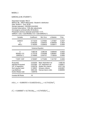
7. MODEL 2
GARCH(1,1), AR(2),
Dependent Variable: RKLCI
Method: ML - ARCH (Marquardt) - Student's t distribution
Date: 05/28/13 Time: 01:06
Sample (adjusted): 1/06/2000 6/24/2005
Included observations: 1335 after adjustments
Convergence achieved after 18 iterations
Presample variance: backcast (parameter = 0.7)
GARCH = C(4) + C(5)*RESID(-1)^2 + C(6)*GARCH(-1)
Variable Coefficient Std. Error z-Statistic Prob.
GARCH 8.307812 4.805453 1.728830 0.0838
C -0.000594 0.000406 -1.462378 0.1436
AR(2) 0.047582 0.028183 1.688309 0.0914
Variance Equation
C 9.90E-06 2.54E-06 3.896075 0.0001
RESID(-1)^2 0.198226 0.038539 5.143464 0.0000
GARCH(-1) 0.703692 0.048270 14.57825 0.0000
T-DIST. DOF 5.449148 0.711329 7.660515 0.0000
R-squared -0.001005 Mean dependent var 7.20E-05
Adjusted R-squared -0.002508 S.D. dependent var 0.009905
S.E. of regression 0.009917 Akaike info criterion -6.652891
Sum squared resid 0.131007 Schwarz criterion -6.625642
Log likelihood 4447.805 Hannan-Quinn criter. -6.642681
Durbin-Watson stat 1.611947
Inverted AR Roots .22 -.22

8. Date: 05/28/13 Time: 01:09
Sample: 1/06/2000 6/24/2005
Included observations: 1335
Q-statistic
probabilities adjusted
for 1 ARMA term(s)
Autocorrelation Partial Correlation AC PAC Q-Stat Prob
|* | |* | 1 0.177 0.177 41.968
| | | | 2 0.039 0.008 44.011 0.000
| | | | 3 0.002 -0.007 44.015 0.000
| | | | 4 0.009 0.010 44.131 0.000
| | | | 5 0.005 0.002 44.165 0.000
| | | | 6 0.037 0.037 46.049 0.000
| | | | 7 0.028 0.016 47.119 0.000
| | | | 8 0.064 0.056 52.593 0.000
| | | | 9 0.019 -0.002 53.076 0.000
| | | | 10 0.024 0.019 53.845 0.000
| | | | 11 0.008 0.001 53.940 0.000
| | | | 12 -0.042 -0.049 56.336 0.000
*| | *| | 13 -0.118 -0.107 74.985 0.000
| | | | 14 -0.026 0.010 75.903 0.000
| | | | 15 -0.002 0.003 75.909 0.000
| | | | 16 0.007 0.002 75.976 0.000
| | | | 17 0.006 0.004 76.017 0.000
| | | | 18 0.041 0.042 78.293 0.000
| | | | 19 0.007 0.002 78.369 0.000
| | | | 20 -0.017 -0.013 78.768 0.000
| | | | 21 0.014 0.035 79.053 0.000
| | | | 22 -0.008 -0.014 79.150 0.000
| | | | 23 -0.005 0.002 79.179 0.000
| | | | 24 0.046 0.047 82.008 0.000
| | | | 25 0.055 0.031 86.093 0.000
| | | | 26 0.035 0.001 87.777 0.000
| | | | 27 0.013 0.002 88.024 0.000
| | | | 28 0.020 0.018 88.545 0.000
| | | | 29 -0.020 -0.032 89.113 0.000
| | | | 30 -0.005 0.003 89.145 0.000
| | | | 31 -0.006 0.001 89.189 0.000
| | | | 32 0.021 0.015 89.798 0.000
| | | | 33 0.034 0.021 91.341 0.000
| | | | 34 -0.003 -0.014 91.354 0.000
| | | | 35 0.024 0.023 92.143 0.000
| | | | 36 -0.002 -0.013 92.148 0.000
Ujian residual diagnostics Q- stat menunjukkakan pada Q(12) nilai probability adalah lebih kecil daripada
0.05, oleh itu menolak H null, ini menunjukkan wujud autokorelasi dalam model.

9. Date: 05/28/13 Time: 01:09
Sample: 1/06/2000 6/24/2005
Included observations: 1335
Q-statistic
probabilities adjusted
for 1 ARMA term(s)
Autocorrelation Partial Correlation AC PAC Q-Stat Prob
| | | | 1 0.009 0.009 0.1153
| | | | 2 0.012 0.011 0.2938 0.588
| | | | 3 -0.009 -0.010 0.4101 0.815
| | | | 4 -0.024 -0.024 1.2018 0.753
| | | | 5 -0.019 -0.019 1.6967 0.791
| | | | 6 -0.011 -0.011 1.8701 0.867
| | | | 7 -0.028 -0.028 2.9208 0.819
| | | | 8 -0.025 -0.025 3.7550 0.808
| | | | 9 0.007 0.007 3.8280 0.872
| | | | 10 -0.013 -0.014 4.0433 0.909
| | | | 11 -0.000 -0.002 4.0434 0.945
| | | | 12 -0.019 -0.021 4.5312 0.952
| | | | 13 0.043 0.042 6.9884 0.858
| | | | 14 -0.010 -0.012 7.1217 0.896
| | | | 15 -0.009 -0.012 7.2327 0.925
| | | | 16 0.045 0.045 9.9707 0.822
| | | | 17 -0.006 -0.006 10.019 0.866
| | | | 18 -0.012 -0.013 10.212 0.894
| | | | 19 0.049 0.050 13.470 0.763
| | | | 20 0.027 0.029 14.454 0.757
| | | | 21 0.003 0.004 14.469 0.806
|* | |* | 22 0.086 0.085 24.560 0.267
| | | | 23 -0.002 0.003 24.564 0.318
| | | | 24 0.032 0.035 25.973 0.302
| | | | 25 0.001 0.005 25.974 0.355
| | | | 26 -0.034 -0.029 27.589 0.327
| | | | 27 -0.002 0.007 27.597 0.379
| | | | 28 0.030 0.038 28.792 0.371
| | | | 29 0.035 0.037 30.474 0.341
| | | | 30 0.065 0.071 36.330 0.164
| | | | 31 0.004 0.008 36.355 0.197
| | | | 32 -0.032 -0.033 37.733 0.189
| | | | 33 0.009 0.012 37.835 0.220
| | | | 34 -0.009 0.002 37.947 0.254
| | | | 35 -0.004 -0.011 37.972 0.293
| | | | 36 0.007 0.012 38.032 0.333
Ujian residual diagnostics Q2
- stat menunjukkakan pada Q(12) nilai probability adalah lebih besar
daripada 0.05, oleh itu gagal menolak H null, ini menunjukkan varians adalah mencukupi.

10. Heteroskedasticity Test: ARCH
F-statistic 0.114795 Prob. F(1,1332) 0.7348
Obs*R-squared 0.114958 Prob. Chi-Square(1) 0.7346
Test Equation:
Dependent Variable: WGT_RESID^2
Method: Least Squares
Date: 05/28/13 Time: 01:09
Sample (adjusted): 1/11/2000 6/24/2005
Included observations: 1334 after adjustments
Variable Coefficient Std. Error t-Statistic Prob.
C 1.012694 0.077069 13.14016 0.0000
WGT_RESID^2(-1) 0.009283 0.027397 0.338814 0.7348
R-squared 0.000086 Mean dependent var 1.022179
Adjusted R-squared -0.000665 S.D. dependent var 2.621713
S.E. of regression 2.622584 Akaike info criterion 4.767695
Sum squared resid 9161.422 Schwarz criterion 4.775485
Log likelihood -3178.053 Hannan-Quinn criter. 4.770614
F-statistic 0.114795 Durbin-Watson stat 1.999556
Prob(F-statistic) 0.734803
H0 : varians adalah homogenous
H1 : varian adalah heterosdastisiti.
Jadual di atas menunjukkan nilai-p chi square adalah lebih besar dari 0.05,oleh itu gagal menolak H null,
ini menunjukkan tidak wujud heterosdastisiti dalam model.

11. Model 3 egarach (1,1)
Dependent Variable: RKLCI
Method: ML - ARCH (Marquardt) - Normal distribution
Date: 05/29/13 Time: 23:14
Sample (adjusted): 1/05/2000 6/24/2005
Included observations: 1336 after adjustments
Convergence achieved after 61 iterations
Presample variance: backcast (parameter = 0.7)
LOG(GARCH) = C(4) + C(5)*ABS(RESID(-1)/@SQRT(GARCH(-1))) + C(6)
*RESID(-1)/@SQRT(GARCH(-1)) + C(7)*LOG(GARCH(-1))
Variable Coefficient Std. Error z-Statistic Prob.
GARCH 5.786282 6.387819 0.905831 0.3650
C -0.000363 0.000511 -0.709683 0.4779
AR(1) 0.204524 0.027271 7.499597 0.0000
Variance Equation
C(4) -0.504055 0.073644 -6.844449 0.0000
C(5) 0.174643 0.018649 9.364513 0.0000
C(6) -0.074039 0.012047 -6.146006 0.0000
C(7) 0.960896 0.007491 128.2706 0.0000
R-squared 0.037028 Mean dependent var 5.65E-05
Adjusted R-squared 0.035584 S.D. dependent var 0.009917
S.E. of regression 0.009739 Akaike info criterion -6.614900
Sum squared resid 0.126441 Schwarz criterion -6.587668
Log likelihood 4425.753 Hannan-Quinn criter. -6.604696
Durbin-Watson stat 2.023557
Inverted AR Roots .20

12. Date: 05/30/13 Time: 00:22
Sample: 1/05/2000 6/24/2005
Included observations: 1336
Q-statistic
probabilities adjusted
for 1 ARMA term(s)
Autocorrelation Partial Correlation AC PAC Q-Stat Prob
| | | | 1 0.016 0.016 0.3636
| | | | 2 0.044 0.043 2.9057 0.088
| | | | 3 -0.006 -0.007 2.9506 0.229
| | | | 4 0.025 0.023 3.7619 0.288
| | | | 5 -0.003 -0.004 3.7780 0.437
| | | | 6 0.037 0.035 5.6122 0.346
| | | | 7 0.011 0.011 5.7900 0.447
|* | |* | 8 0.078 0.074 13.969 0.052
| | | | 9 -0.006 -0.008 14.011 0.081
| | | | 10 0.027 0.019 14.960 0.092
| | | | 11 0.001 0.002 14.961 0.133
| | | | 12 -0.022 -0.029 15.611 0.156
*| | *| | 13 -0.096 -0.096 28.188 0.005
| | | | 14 0.002 0.000 28.192 0.009
| | | | 15 -0.009 -0.003 28.307 0.013
| | | | 16 0.013 0.006 28.536 0.018
| | | | 17 -0.008 -0.003 28.615 0.027
| | | | 18 0.050 0.048 31.970 0.015
| | | | 19 0.007 0.014 32.040 0.022
| | | | 20 -0.011 -0.010 32.198 0.030
| | | | 21 0.016 0.031 32.546 0.038
| | | | 22 0.000 -0.002 32.546 0.051
| | | | 23 -0.007 -0.004 32.609 0.068
| | | | 24 0.040 0.037 34.792 0.055
| | | | 25 0.040 0.033 36.950 0.044
| | | | 26 0.025 0.005 37.822 0.048
| | | | 27 -0.009 -0.014 37.934 0.061
| | | | 28 0.034 0.031 39.497 0.057
| | | | 29 -0.016 -0.022 39.867 0.068
| | | | 30 -0.003 -0.007 39.882 0.086
Ujian residual diagnostics Q- stat menunjukkakan pada Q(12) nilai probability adalah lebih kecil daripada
0.05, oleh itu gagal menolak H null, ini menunjukkan wujud tidak autokorelasi dalam model.

13. Date: 05/30/13 Time: 00:25
Sample: 1/05/2000 6/24/2005
Included observations: 1336
Q-statistic
probabilities adjusted
for 1 ARMA term(s)
Autocorrelation Partial Correlation AC PAC Q-Stat Prob
| | | | 1 0.059 0.059 4.6619
| | | | 2 0.063 0.059 9.9385 0.002
| | | | 3 0.010 0.003 10.060 0.007
| | | | 4 -0.013 -0.018 10.295 0.016
| | | | 5 -0.029 -0.029 11.462 0.022
| | | | 6 -0.011 -0.006 11.619 0.040
| | | | 7 -0.030 -0.025 12.803 0.046
| | | | 8 -0.044 -0.040 15.430 0.031
| | | | 9 0.008 0.015 15.517 0.050
| | | | 10 -0.031 -0.028 16.812 0.052
| | | | 11 -0.020 -0.019 17.345 0.067
| | | | 12 -0.031 -0.028 18.612 0.068
| | | | 13 0.019 0.023 19.103 0.086
| | | | 14 -0.020 -0.020 19.651 0.104
| | | | 15 -0.016 -0.020 19.979 0.131
| | | | 16 0.028 0.029 21.044 0.135
| | | | 17 -0.036 -0.039 22.768 0.120
| | | | 18 -0.032 -0.035 24.181 0.115
| | | | 19 0.034 0.038 25.708 0.107
| | | | 20 0.010 0.009 25.845 0.135
| | | | 21 -0.011 -0.016 26.010 0.165
| | | | 22 0.063 0.056 31.453 0.066
| | | | 23 0.020 0.015 31.982 0.078
| | | | 24 -0.001 -0.010 31.985 0.100
| | | | 25 -0.018 -0.026 32.449 0.116
| | | | 26 -0.030 -0.026 33.652 0.116
| | | | 27 -0.019 -0.006 34.129 0.132
| | | | 28 0.044 0.049 36.732 0.100
| | | | 29 0.033 0.029 38.227 0.094
| | | | 30 0.059 0.058 42.996 0.046
| | | | 31 -0.008 -0.019 43.081 0.058
| | *| | 32 -0.056 -0.068 47.410 0.030
| | | | 33 -0.023 -0.012 48.156 0.033
| | | | 34 -0.023 -0.006 48.889 0.037
| | | | 35 -0.029 -0.028 50.026 0.038
| | | | 36 -0.007 0.003 50.090 0.047
Ujian residual diagnostics Q2
- stat menunjukkakan pada Q(12) nilai probability adalah lebih besar
daripada 0.05, oleh itu gagal menolak H null, ini menunjukkan varians adalah mencukupi.

14. Heteroskedasticity Test: ARCH
F-statistic 4.657425 Prob. F(1,1333) 0.0311
Obs*R-squared 4.648172 Prob. Chi-Square(1) 0.0311
Test Equation:
Dependent Variable: WGT_RESID^2
Method: Least Squares
Date: 05/30/13 Time: 00:30
Sample (adjusted): 1/06/2000 6/24/2005
Included observations: 1335 after adjustments
Variable Coefficient Std. Error t-Statistic Prob.
C 0.933735 0.062752 14.87988 0.0000
WGT_RESID^2(-1) 0.059007 0.027342 2.158107 0.0311
R-squared 0.003482 Mean dependent var 0.992317
Adjusted R-squared 0.002734 S.D. dependent var 2.070005
S.E. of regression 2.067173 Akaike info criterion 4.291738
Sum squared resid 5696.184 Schwarz criterion 4.299524
Log likelihood -2862.735 Hannan-Quinn criter. 4.294656
F-statistic 4.657425 Durbin-Watson stat 2.006772
Prob(F-statistic) 0.031098
H0 : varians adalah homogenous
H1 : varian adalah heterosdastisiti.
Jadual di atas menunjukkan nilai-p chi square adalah lebih kecil dari 0.05,oleh itu menolak H null, ini
menunjukkan wujud heterosdastisiti dalam model.

15. Model 4 EGARCH(1,1)
Dependent Variable: RKLCI
Method: ML - ARCH (Marquardt) - Student's t distribution
Date: 05/30/13 Time: 00:53
Sample (adjusted): 1/05/2000 6/24/2005
Included observations: 1336 after adjustments
Convergence achieved after 19 iterations
Presample variance: backcast (parameter = 0.7)
LOG(GARCH) = C(4) + C(5)*ABS(RESID(-1)/@SQRT(GARCH(-1))) + C(6)
*RESID(-1)/@SQRT(GARCH(-1)) + C(7)*LOG(GARCH(-1))
Variable Coefficient Std. Error z-Statistic Prob.
GARCH 6.095233 5.466759 1.114963 0.2649
C -0.000525 0.000442 -1.187902 0.2349
AR(1) 0.166727 0.027819 5.993372 0.0000
Variance Equation
C(4) -0.926758 0.207993 -4.455728 0.0000
C(5) 0.277872 0.045509 6.105849 0.0000
C(6) -0.070588 0.025550 -2.762772 0.0057
C(7) 0.924446 0.020246 45.66077 0.0000
T-DIST. DOF 5.891519 0.869331 6.777073 0.0000
R-squared 0.035912 Mean dependent var 5.65E-05
Adjusted R-squared 0.034466 S.D. dependent var 0.009917
S.E. of regression 0.009745 Akaike info criterion -6.679959
Sum squared resid 0.126588 Schwarz criterion -6.648837
Log likelihood 4470.213 Hannan-Quinn criter. -6.668298
Durbin-Watson stat 1.939539
Inverted AR Roots .17

16. Date: 05/30/13 Time: 00:59
Sample: 1/05/2000 6/24/2005
Included observations: 1336
Q-statistic
probabilities adjusted
for 1 ARMA term(s)
Autocorrelation Partial Correlation AC PAC Q-Stat Prob
| | | | 1 0.056 0.056 4.1261
| | | | 2 0.054 0.051 8.0690 0.005
| | | | 3 -0.001 -0.007 8.0702 0.018
| | | | 4 0.019 0.016 8.5378 0.036
| | | | 5 -0.001 -0.003 8.5405 0.074
| | | | 6 0.038 0.037 10.508 0.062
| | | | 7 0.015 0.012 10.818 0.094
| | | | 8 0.072 0.067 17.857 0.013
| | | | 9 0.002 -0.006 17.862 0.022
| | | | 10 0.022 0.014 18.495 0.030
| | | | 11 0.001 -0.001 18.496 0.047
| | | | 12 -0.025 -0.030 19.319 0.056
*| | *| | 13 -0.103 -0.102 33.663 0.001
| | | | 14 -0.005 0.002 33.699 0.001
| | | | 15 -0.009 -0.000 33.804 0.002
| | | | 16 0.009 0.004 33.926 0.003
| | | | 17 -0.004 -0.002 33.950 0.006
| | | | 18 0.044 0.043 36.518 0.004
| | | | 19 0.005 0.009 36.549 0.006
| | | | 20 -0.014 -0.013 36.807 0.008
| | | | 21 0.015 0.031 37.115 0.011
| | | | 22 -0.002 -0.004 37.121 0.016
| | | | 23 -0.007 -0.006 37.194 0.023
| | | | 24 0.038 0.036 39.158 0.019
| | | | 25 0.042 0.033 41.512 0.015
| | | | 26 0.028 0.004 42.552 0.016
| | | | 27 -0.001 -0.008 42.553 0.022
| | | | 28 0.031 0.029 43.840 0.021
| | | | 29 -0.017 -0.023 44.215 0.026
| | | | 30 -0.007 -0.010 44.285 0.034
| | | | 31 -0.011 -0.003 44.465 0.043
| | | | 32 0.017 0.011 44.843 0.051
| | | | 33 0.030 0.024 46.047 0.052
| | | | 34 -0.006 -0.011 46.097 0.065
| | | | 35 0.026 0.025 47.029 0.068
| | | | 36 0.001 -0.006 47.030 0.084
Ujian residual diagnostics Q- stat menunjukkakan pada Q(12) nilai probability adalah lebih besar
daripada 0.05, oleh itu gagal menolak H null, ini menunjukkan tidak wujud autokorelasi dalam model.

17. Date: 05/30/13 Time: 01:01
Sample: 1/05/2000 6/24/2005
Included observations: 1336
Q-statistic
probabilities adjusted
for 1 ARMA term(s)
Autocorrelation Partial Correlation AC PAC Q-Stat Prob
| | | | 1 0.021 0.021 0.5643
| | | | 2 0.040 0.039 2.6851 0.101
| | | | 3 -0.009 -0.011 2.8015 0.246
| | | | 4 -0.024 -0.025 3.5732 0.311
| | | | 5 -0.033 -0.031 5.0133 0.286
| | | | 6 -0.015 -0.012 5.3255 0.377
| | | | 7 -0.031 -0.028 6.5804 0.361
| | | | 8 -0.038 -0.038 8.5641 0.285
| | | | 9 0.007 0.009 8.6314 0.374
| | | | 10 -0.025 -0.025 9.4901 0.393
| | | | 11 -0.010 -0.013 9.6325 0.473
| | | | 12 -0.025 -0.026 10.462 0.489
| | | | 13 0.032 0.031 11.838 0.459
| | | | 14 -0.014 -0.016 12.109 0.519
| | | | 15 -0.013 -0.020 12.355 0.578
| | | | 16 0.040 0.039 14.468 0.490
| | | | 17 -0.018 -0.020 14.924 0.530
| | | | 18 -0.024 -0.029 15.719 0.544
| | | | 19 0.048 0.049 18.902 0.398
| | | | 20 0.019 0.019 19.412 0.431
| | | | 21 -0.010 -0.013 19.542 0.487
|* | |* | 22 0.081 0.076 28.394 0.129
| | | | 23 0.018 0.019 28.815 0.150
| | | | 24 0.012 0.009 28.998 0.180
| | | | 25 -0.007 -0.007 29.056 0.218
| | | | 26 -0.032 -0.027 30.424 0.209
| | | | 27 -0.009 0.004 30.533 0.246
| | | | 28 0.042 0.050 32.989 0.197
| | | | 29 0.040 0.040 35.143 0.166
| | | | 30 0.068 0.073 41.507 0.062
Ujian residual diagnostics Q2
- stat menunjukkakan pada Q(12) nilai probability adalah lebih besar
daripada 0.05, oleh itu gagal menolak H null, ini menunjukkan varians adalah mencukupi.

18. Heteroskedasticity Test: ARCH
F-statistic 0.562067 Prob. F(1,1333) 0.4536
Obs*R-squared 0.562673 Prob. Chi-Square(1) 0.4532
Test Equation:
Dependent Variable: WGT_RESID^2
Method: Least Squares
Date: 05/30/13 Time: 01:02
Sample (adjusted): 1/06/2000 6/24/2005
Included observations: 1335 after adjustments
Variable Coefficient Std. Error t-Statistic Prob.
C 0.987383 0.067415 14.64644 0.0000
WGT_RESID^2(-1) 0.020530 0.027384 0.749711 0.4536
R-squared 0.000421 Mean dependent var 1.008090
Adjusted R-squared -0.000328 S.D. dependent var 2.246574
S.E. of regression 2.246943 Akaike info criterion 4.458515
Sum squared resid 6729.987 Schwarz criterion 4.466301
Log likelihood -2974.059 Hannan-Quinn criter. 4.461432
F-statistic 0.562067 Durbin-Watson stat 2.001382
Prob(F-statistic) 0.453561
H0 : varians adalah homogenous
H1 : varian adalah heterosdastisiti.
Jadual di atas menunjukkan nilai-p chi square adalah lebih besar dari 0.05,oleh itu gagal menolak H null,
ini menunjukkan tidak wujud heterosdastisiti dalam model.

19. Model 5 GARCH(1,1) LOG-VAR
Dependent Variable: RKLCI
Method: ML - ARCH (Marquardt) - Student's t distribution
Date: 05/30/13 Time: 01:54
Sample (adjusted): 1/05/2000 6/24/2005
Included observations: 1336 after adjustments
Convergence achieved after 23 iterations
Presample variance: backcast (parameter = 0.7)
GARCH = C(4) + C(5)*RESID(-1)^2 + C(6)*GARCH(-1)
Variable Coefficient Std. Error z-Statistic Prob.
LOG(GARCH) 0.001104 0.000558 1.978373 0.0479
C 0.010779 0.005434 1.983393 0.0473
AR(1) 0.155840 0.028965 5.380234 0.0000
Variance Equation
C 8.92E-06 2.32E-06 3.848522 0.0001
RESID(-1)^2 0.191628 0.037558 5.102223 0.0000
GARCH(-1) 0.717005 0.045888 15.62498 0.0000
T-DIST. DOF 5.796714 0.774819 7.481376 0.0000
R-squared 0.032428 Mean dependent var 5.65E-05
Adjusted R-squared 0.030976 S.D. dependent var 0.009917
S.E. of regression 0.009763 Akaike info criterion -6.672274
Sum squared resid 0.127045 Schwarz criterion -6.645042
Log likelihood 4464.079 Hannan-Quinn criter. -6.662071
Durbin-Watson stat 1.929307
Inverted AR Roots .16

20. Date: 05/30/13 Time: 02:00
Sample: 1/05/2000 6/24/2005
Included observations: 1336
Q-statistic
probabilities adjusted
for 1 ARMA term(s)
Autocorrelation Partial Correlation AC PAC Q-Stat Prob
| | | | 1 0.040 0.040 2.1203
| | | | 2 0.047 0.046 5.1334 0.023
| | | | 3 -0.006 -0.010 5.1844 0.075
| | | | 4 0.008 0.006 5.2669 0.153
| | | | 5 0.002 0.003 5.2740 0.260
| | | | 6 0.036 0.036 7.0425 0.217
| | | | 7 0.019 0.017 7.5500 0.273
| | | | 8 0.068 0.064 13.843 0.054
| | | | 9 0.012 0.006 14.038 0.081
| | | | 10 0.035 0.028 15.664 0.074
| | | | 11 0.016 0.014 16.012 0.099
| | | | 12 -0.021 -0.027 16.611 0.120
*| | *| | 13 -0.102 -0.103 30.595 0.002
| | | | 14 -0.003 0.001 30.607 0.004
| | | | 15 0.003 0.009 30.620 0.006
| | | | 16 0.013 0.005 30.861 0.009
| | | | 17 0.000 -0.003 30.861 0.014
| | | | 18 0.045 0.043 33.577 0.010
| | | | 19 0.003 0.006 33.592 0.014
| | | | 20 -0.017 -0.016 33.965 0.019
| | | | 21 0.020 0.034 34.488 0.023
| | | | 22 -0.006 -0.005 34.534 0.032
| | | | 23 -0.002 0.001 34.537 0.043
| | | | 24 0.048 0.050 37.740 0.027
| | | | 25 0.053 0.044 41.510 0.015
| | | | 26 0.035 0.011 43.178 0.013
| | | | 27 0.012 0.004 43.371 0.018
| | | | 28 0.028 0.027 44.458 0.019
| | | | 29 -0.017 -0.024 44.836 0.023
| | | | 30 0.000 -0.003 44.837 0.031
| | | | 31 -0.003 0.002 44.849 0.040
| | | | 32 0.021 0.011 45.466 0.045
| | | | 33 0.035 0.024 47.162 0.041
| | | | 34 -0.006 -0.013 47.206 0.052
| | | | 35 0.034 0.027 48.791 0.048
| | | | 36 -0.000 -0.008 48.791 0.061
Ujian residual diagnostics Q- stat menunjukkakan pada Q(12) nilai probability adalah lebih besar
daripada 0.05, oleh itu gagal menolak H null, ini menunjukkan tidak wujud autokorelasi dalam model.

21. Date: 05/30/13 Time: 02:01
Sample: 1/05/2000 6/24/2005
Included observations: 1336
Q-statistic
probabilities adjusted
for 1 ARMA term(s)
Autocorrelation Partial Correlation AC PAC Q-Stat Prob
| | | | 1 -0.001 -0.001 0.0016
| | | | 2 0.013 0.013 0.2235 0.636
| | | | 3 -0.010 -0.010 0.3483 0.840
| | | | 4 -0.027 -0.027 1.3220 0.724
| | | | 5 -0.031 -0.031 2.6134 0.624
| | | | 6 -0.008 -0.007 2.6943 0.747
| | | | 7 -0.029 -0.029 3.8482 0.697
| | | | 8 -0.019 -0.020 4.3403 0.740
| | | | 9 0.007 0.006 4.4007 0.819
| | | | 10 -0.020 -0.022 4.9549 0.838
| | | | 11 -0.008 -0.011 5.0412 0.888
| | | | 12 -0.016 -0.019 5.4042 0.910
| | | | 13 0.037 0.035 7.2558 0.840
| | | | 14 -0.009 -0.011 7.3645 0.882
| | | | 15 -0.007 -0.012 7.4379 0.917
| | | | 16 0.037 0.036 9.2932 0.862
| | | | 17 -0.008 -0.008 9.3869 0.897
| | | | 18 -0.022 -0.023 10.020 0.903
| | | | 19 0.042 0.042 12.412 0.825
| | | | 20 0.039 0.042 14.441 0.757
| | | | 21 -0.006 -0.005 14.486 0.805
|* | |* | 22 0.085 0.082 24.201 0.283
| | | | 23 -0.001 0.005 24.203 0.337
| | | | 24 0.038 0.042 26.132 0.295
| | | | 25 0.007 0.011 26.194 0.343
| | | | 26 -0.040 -0.035 28.418 0.289
| | | | 27 -0.002 0.009 28.426 0.338
| | | | 28 0.051 0.058 31.917 0.235
| | | | 29 0.037 0.042 33.740 0.210
| | | | 30 0.063 0.069 39.127 0.099
| | | | 31 -0.002 0.003 39.133 0.123
| | | | 32 -0.036 -0.033 40.920 0.110
| | | | 33 -0.005 -0.001 40.955 0.133
| | | | 34 -0.013 0.001 41.180 0.155
| | | | 35 -0.003 -0.004 41.197 0.185
| | | | 36 0.000 0.003 41.197 0.218
Ujian residual diagnostics Q2
- stat menunjukkakan pada Q(12) nilai probability adalah lebih besar
daripada 0.05, oleh itu gagal menolak H null, ini menunjukkan varians adalah mencukupi.

22. Heteroskedasticity Test: ARCH
F-statistic 0.001608 Prob. F(1,1333) 0.9680
Obs*R-squared 0.001610 Prob. Chi-Square(1) 0.9680
Test Equation:
Dependent Variable: WGT_RESID^2
Method: Least Squares
Date: 05/30/13 Time: 02:02
Sample (adjusted): 1/06/2000 6/24/2005
Included observations: 1335 after adjustments
Variable Coefficient Std. Error t-Statistic Prob.
C 1.047624 0.077247 13.56206 0.0000
WGT_RESID^2(-1) -0.001098 0.027391 -0.040097 0.9680
R-squared 0.000001 Mean dependent var 1.046474
Adjusted R-squared -0.000749 S.D. dependent var 2.619654
S.E. of regression 2.620635 Akaike info criterion 4.766207
Sum squared resid 9154.678 Schwarz criterion 4.773992
Log likelihood -3179.443 Hannan-Quinn criter. 4.769124
F-statistic 0.001608 Durbin-Watson stat 1.999780
Prob(F-statistic) 0.968022
H0 : varians adalah homogenous
H1 : varian adalah heterosdastisiti.
Jadual di atas menunjukkan nilai-p chi square adalah lebih besar dari 0.05,oleh itu gagal menolak H null,
ini menunjukkan tidak wujud heterosdastisiti dalam model.