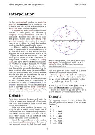
1. From Wikipedia, the free encyclopedia Interpolation
Interpolation
In the mathematical subfield of numerical
analysis, interpolation is a method of con-
structing new data points within the range of
a discrete set of known data points.
In engineering and science one often has a
number of data points, as obtained by
sampling or experimentation, and tries to
construct a function which closely fits those
data points. This is called curve fitting or re-
gression analysis. Interpolation is a specific
case of curve fitting, in which the function
must go exactly through the data points.
A different problem which is closely re-
lated to interpolation is the approximation of
a complicated function by a simple function.
Suppose we know the function but it is too
complex to evaluate efficiently. Then we
could pick a few known data points from the
complicated function, creating a lookup An interpolation of a finite set of points on an
table, and try to interpolate those data points epitrochoid. Points through which curve is
to construct a simpler function. Of course, splined are red; the blue curve connecting
when using the simple function to calculate them is interpolation.
new data points we usually do not receive the
same result as when using the original func- This will give the same result as a linear
tion, but depending on the problem domain function evaluated at the midpoint.
and the interpolation method used the gain in Given a sequence of n distinct numbers xk
simplicity might offset the error. called nodes and for each xk a second num-
It should be mentioned that there is anoth- ber yk, we are looking for a function f so that
er very different kind of interpolation in
mathematics, namely the "interpolation of op-
erators". The classical results about interpol-
A pair xk,yk is called a data point and f is
ation of operators are the Riesz-Thorin theor-
called an interpolant for the data points.
em and the Marcinkiewicz theorem. There
When the numbers yk are given by a
also are many other subsequent results.
known function f, we sometimes write fk.
Definition Example
From inter meaning between and pole, the
For example, suppose we have a table like
points or nodes. Any means of calculating a
this, which gives some values of an unknown
new point between two or more existing data
function f.
points is interpolation.
x f(x)
There are many methods for doing this,
many of which involve fitting some sort of 0 0
function to the data and evaluating that func- 1 0 . 8415
tion at the desired point. This does not ex- 2 0 . 9093
clude other means such as statistical meth- 3 0 . 1411
ods of calculating interpolated data. 4 −0 . 7568
One of the simplest forms of interpolation
5 −0 . 9589
is to take the arithmetic mean of the value of
6 −0 . 2794
two adjacent points to find the mid point.
1

2. From Wikipedia, the free encyclopedia Interpolation
but in higher dimensions, in multivariate in-
terpolation, this can be a favourable choice
for its speed and simplicity.
Linear interpolation
Plot of the data points as given in the table.
Interpolation provides a means of estimating
the function at intermediate points, such as
x = 2.5.
There are many different interpolation
Plot of the data with linear interpolation
methods, some of which are described below.
superimposed
Some of the concerns to take into account
when choosing an appropriate algorithm are:
One of the simplest methods is linear inter-
How accurate is the method? How expensive
polation (sometimes known as lerp). Consider
is it? How smooth is the interpolant? How
the above example of determining f(2.5).
many data points are needed?
Since 2.5 is midway between 2 and 3, it is
reasonable to take f(2.5) midway between
Piecewise constant f(2) = 0.9093 and f(3) = 0.1411, which yields
0.5252.
interpolation Generally, linear interpolation takes two
data points, say (xa,ya) and (xb,yb), and the
interpolant is given by:
at the
point (x,y)
Linear interpolation is quick and easy, but it
is not very precise. Another disadvantage is
that the interpolant is not differentiable at
the point xk.
The following error estimate shows that
linear interpolation is not very precise. De-
note the function which we want to interpol-
ate by g, and suppose that x lies between xa
Piecewise constant interpolation, or nearest- and xb and that g is twice continuously differ-
neighbor interpolation. entiable. Then the linear interpolation error
is
For more details on this topic, see Nearest-
neighbor interpolation.
The simplest interpolation method is to loc-
ate the nearest data value, and assign the In words, the error is proportional to the
same value. In one dimension, there are sel- square of the distance between the data
dom good reasons to choose this one over lin- points. The error of some other methods, in-
ear interpolation, which is almost as cheap, cluding polynomial interpolation and spline
2

3. From Wikipedia, the free encyclopedia Interpolation
interpolation (described below), is propor- Runge’s phenomenon). These disadvantages
tional to higher powers of the distance can be avoided by using spline interpolation.
between the data points. These methods also
produce smoother interpolants.
Spline interpolation
Polynomial interpolation
Plot of the data with Spline interpolation
applied
Plot of the data with polynomial interpolation
applied Remember that linear interpolation uses a
linear function for each of intervals [xk,xk+1].
Polynomial interpolation is a generalization Spline interpolation uses low-degree polyno-
of linear interpolation. Note that the linear mials in each of the intervals, and chooses
interpolant is a linear function. We now re- the polynomial pieces such that they fit
place this interpolant by a polynomial of smoothly together. The resulting function is
higher degree. called a spline.
Consider again the problem given above. For instance, the natural cubic spline is
The following sixth degree polynomial goes piecewise cubic and twice continuously dif-
through all the seven points: ferentiable. Furthermore, its second derivat-
f(x) = − 0.0001521x6 − 0.003130x5 + ive is zero at the end points. The natural cu-
0.07321x4 − 0.3577x3 + 0.2255x2 + bic spline interpolating the points in the table
0.9038x. above is given by
Substituting x = 2.5, we find that f(2.5) =
0.5965.
Generally, if we have n data points, there
is exactly one polynomial of degree at most
n−1 going through all the data points. The in- In this case we get f(2.5)=0.5972.
terpolation error is proportional to the dis- Like polynomial interpolation, spline inter-
tance between the data points to the power polation incurs a smaller error than linear in-
n. Furthermore, the interpolant is a polyno- terpolation and the interpolant is smoother.
mial and thus infinitely differentiable. So, we However, the interpolant is easier to evaluate
see that polynomial interpolation solves all than the high-degree polynomials used in
the problems of linear interpolation. polynomial interpolation. It also does not suf-
However, polynomial interpolation also fer from Runge’s phenomenon.
has some disadvantages. Calculating the in-
terpolating polynomial is computationally ex-
pensive (see computational complexity) com- Interpolation via Gaussi-
pared to linear interpolation. Furthermore,
polynomial interpolation may not be so exact
an processes
after all, especially at the end points (see Gaussian process is a powerful non-linear in-
terpolation tool. Many popular interpolation
tools are actually equivalent to particular
3

4. From Wikipedia, the free encyclopedia Interpolation
Gaussian processes. Gaussian processes can In curve fitting problems, the constraint
be used not only for fitting an interpolant that the interpolant has to go exactly through
that passes exactly through the given data the data points is relaxed. It is only required
points but also for regression, i.e. for fitting a to approach the data points as closely as pos-
curve through noisy data. In the geostatistics sible. This requires parameterizing the poten-
community Gaussian process regression is tial interpolants and having some way of
also known as Kriging. measuring the error. In the simplest case this
leads to least squares approximation.
Other forms of Approximation theory studies how to find
the best approximation to a given function by
interpolation another function from some predetermined
class, and how good this approximation is.
Other forms of interpolation can be construc-
This clearly yields a bound on how well the
ted by picking a different class of inter-
interpolant can approximate the unknown
polants. For instance, rational interpolation is
function.
interpolation by rational functions, and tri-
gonometric interpolation is interpolation by
trigonometric polynomials. The discrete References
Fourier transform is a special case of trigono- • David Kidner, Mark Dorey and Derek
metric interpolation. Another possibility is to Smith (1999). What’s the point?
use wavelets. Interpolation and extrapolation with a
The Whittaker–Shannon interpolation for- regular grid DEM. IV International
mula can be used if the number of data Conference on GeoComputation,
points is infinite. Fredericksburg, VA, USA.
Multivariate interpolation is the interpola- • Kincaid, David; Ward Cheney (2002).
tion of functions of more than one variable. Numerical Analysis (3rd edition). Brooks/
Methods include bilinear interpolation and Cole. ISBN 0-534-38905-8. Chapter 6.
bicubic interpolation in two dimensions, and • Schatzman, Michelle (2002). Numerical
trilinear interpolation in three dimensions. Analysis: A Mathematical Introduction.
Sometimes, we know not only the value of Clarendon Press, Oxford. ISBN
the function that we want to interpolate, at 0-19-850279-6. Chapters 4 and 6.
some points, but also its derivative. This
leads to Hermite interpolation problems.
External links
Related concepts • DotPlacer applet : Applet showing various
interpolation methods, with movable
The term extrapolation is used if we want to points
find data points outside the range of known
data points.
Retrieved from "http://en.wikipedia.org/wiki/Interpolation"
Categories: Interpolation
This page was last modified on 14 May 2009, at 22:02 (UTC). All text is available under the
terms of the GNU Free Documentation License. (See Copyrights for details.) Wikipedia® is a
registered trademark of the Wikimedia Foundation, Inc., a U.S. registered 501(c)(3) tax-
deductible nonprofit charity. Privacy policy About Wikipedia Disclaimers
4