1. 3D VISUALIZATION OF EARTHQUAKE FOCAL
MECHANISMS USING ARCSCENE®
fgfg
By Keith A. Labay and Peter J. Haeuisler
Any use of trade, firm, or product names is for descriptive purposes only and does not
imply endorseme7t by the U.S. Governme7t
Data Series 241
Version 1.1

2. U.S. Department of the Interior
DIRK KEMPTHORNE, Secretary
U.S. Geological Survey
Mark D. Myers, Director
U.S. Geological Survey, Reston, Virginia 2007
For product and ordering information:
World Wide Web: http://www.usgs.gov/pubprod
Telephone: 1-888-ASK-USGS
For more information on the USGS—the Federal source for science about the Earth,
its natural and living resources, natural hazards, and the environment:
World Wide Web: http://www.usgs.gov
Telephone: 1-888-ASK-USGS
Any use of trade, product, or firm names is for descriptive purposes only and does not imply
endorsement by the U.S. Government.
Although this report is in the public domain, permission must be secured from the individual
copyright owners to reproduce any copyrighted material contained within this report.
Manuscript approved for publication January 3, 2007
2

3. Contents
Abstract .....................................................................................................................................................................................4
1.0 Introduction .........................................................................................................................................................................4
1.1 Purpose ............................................................................................................................................................................4
1.2 Software...........................................................................................................................................................................5
1.3 Focal Mechanisms ...........................................................................................................................................................5
1.4 Setup ................................................................................................................................................................................5
1.5 Input data .........................................................................................................................................................................5
File Types ..........................................................................................................................................................................5
Required Fields..................................................................................................................................................................5
Optional Fields ..................................................................................................................................................................6
Coordinate Systems ...........................................................................................................................................................6
Scene Properties ................................................................................................................................................................7
2.0 Using 3D Focal Mechanisms...............................................................................................................................................8
2.1 ArcScene® ........................................................................................................................................................................8
2.2 Initial Steps ......................................................................................................................................................................8
2.3 Appearance Settings ........................................................................................................................................................9
Symbol Options .................................................................................................................................................................9
Sizing Options .................................................................................................................................................................12
Position Options ..............................................................................................................................................................14
Output Coordinate System...............................................................................................................................................14
2.4 Filter data.......................................................................................................................................................................15
Filtering Options..............................................................................................................................................................15
2.5 Displaying the symbols..................................................................................................................................................16
Output symbol layer ........................................................................................................................................................16
3.0 Example.............................................................................................................................................................................17
4.0 References Cited................................................................................................................................................................17
5.0 Acknowledgments .............................................................................................................................................................17
Figure 1. Screen shot of the 3DFM interface............................................................................................................................4
Figure 2. Example of a point attribute table with required and optional fields.........................................................................6
Figure 3. Screen shot of the Scene Properties window.............................................................................................................7
Figure 4. Screen shot of the Standard toolbar...........................................................................................................................8
Figure 5. Screen shot of the 3DFM interface symbols tab........................................................................................................8
Figure 6. Default focal spheres appearance. .............................................................................................................................9
Figure 7. Nodal planes with rings colored by magnitude. ......................................................................................................10
Figure 8. Focal spheres with rings colored by magnitude. .....................................................................................................10
Figure 9. Primary planes colored by magnitude. ....................................................................................................................11
Figure 10. “Principal Stress Axes” selected as the only symbol option (left), and in combination with the “Nodal Planes”
option (right)....................................................................................................................................................................12
Figure 11. Two views of the same dataset with a different symbol diameter.........................................................................12
Figure 12. Focal spheres scaled by magnitude. ......................................................................................................................13
Figure 13. Focal spheres scaled by rupture patch size. ...........................................................................................................13
Figure 14. Focal spheres of the Benioff zone of southcentral Alaska, with the “View depth” option turned on. Horizontal
line of dots at top corresponds to the Earth’s surface. .....................................................................................................14
Figure 15. Screen shot of the 3DFM interface filter data tab..................................................................................................15
Figure 16. Example image of focal mechanism symbols along the Denali Fault and Susitna Glacier Thrust Fault...............17
Table 1. Magnitude color ranges.............................................................................................................................................11
3

4. Abstract
We created a new tool, 3D Focal Mechanisms (3DFM), for viewing earthquake focal mechanism symbols three dimen-
sionally. This tool operates within the Environmental Systems Research Institute (ESRI®) GIS software ArcScene® 9.x. The
program requires as input a GIS point dataset of earthquake locations containing strike, dip, and rake values for a nodal
plane of each earthquake. Other information, such as depth and magnitude of the earthquake, may also be included in the
dataset. By default for each focal point, 3DFM will create a black and white sphere or “beach ball” that is oriented based on
the strike, dip, and rake values. If depth values for each earthquake are included, the focal symbol will also be placed at its
appropriate location beneath the Earth’s surface.
In addition to the default settings, there are several other options in 3DFM that can be adjusted. The appearance of the
symbols can be changed by (1) creating rings around the fault planes that are colored based on magnitude, (2) showing only
the fault planes instead of a sphere, (3) drawing a flat disc that identifies the primary nodal plane, (4) or by displaying the
null, pressure, and tension axes. The size of the symbols can be changed by adjusting their diameter, scaling them based on
the magnitude of the earthquake, or scaling them by the estimated size of the rupture patch based on earthquake magnitude.
It is also possible to filter the data using any combination of the strike, dip, rake, magnitude, depth, null axis plunge, pres-
sure axis plunge, tension axis plunge, or fault type values of the points. For a large dataset, these filters can be used to create
different subsets of symbols. Symbols created by 3DFM are stored in graphics layers that appear in the ArcScene® table of
contents. Multiple graphics layers can be created and saved to preserve the output from different symbol options.
1.0 Introduction
1.1 Purpose
This tool, 3D Focal Mechanisms (3DFM), is designed to display three-dimensional focal mechanism symbols for
earthquake point locations that have been loaded into the Environmental Systems Research Institute (ESRI®) GIS software
ArcScene® 9.x. A new button has been added to the end of the standard toolbar in the provided ArcScene® file
3DFocalMech.sxd. It will launch an interface from which three-dimensional focal mechanism symbols can be created for
earthquake locations (fig. 1). The tool is primarily intended for use by seismologists or others familiar with interpreting fo-
cal mechanism symbols. 3DFM was created so that viewing three-dimensional (3D) focal mechanism symbols could be
done in a commonly used GIS software package without the need to rely on more specialized software that might not be
compatible with existing datasets. A basic understanding of GIS concepts would be helpful but is not necessary when using
3DFM.
Figure 1. Screen shot of the 3DFM interface.
4

5. 1.2 Software
ArcScene® 9.x is a module within the ArcGIS® 9.x suite of software. It is designed for three-dimensional viewing of
GIS data.
1.3 Focal Mechanisms
The first arrival of seismic waves from an earthquake caused by movement on a fault can be divided into quadrants
showing either compression or dilation (frequently referred to as “tension”). The planes dividing these quadrants are re-
ferred to as nodal planes. One of these planes is the fault plane, and the other is referred to as the auxiliary plane and has no
structural significance. Additional information is needed to determine which of the nodal planes is the fault plane or auxil-
iary plane, such as a geologically mapped fault or an alignment of earthquakes along a plane.
A focal mechanism symbol is a graphical representation of these compressional or dilational quadrants. When viewed
three dimensionally, a focal mechanism symbol can be displayed as a sphere divided into four equal sized diagonally oppos-
ing black and white quadrants. This sphere looks like a beach ball, and sometimes a figure showing focal mechanisms is
referred to as a “beach ball” diagram. The black quadrants represent areas that moved away from the earthquake’s hypocen-
ter, whereas the white quadrants represent areas that moved toward the earthquake’s hypocenter. A two-dimensional focal
mechanism symbol is displayed using a lower hemisphere sterographic projection. This means that the two-dimensional
symbol is showing you what it would look like if a three-dimensional sphere was cut in half along a plane defined by the
surface of the Earth, and then you looked down into the hollow lower half (see for example, Cronin, 2004).
1.4 Setup
1. If ArcScene® 9.x is already installed on the computer no additional software will need to be installed.
2. Download the file: 3DFocalMechanisms.zip
3. Unzip this file to the computer’s hard drive.
This zip file contains the following files:
3DFocalMech – A folder containing two files 3DFM needs to create the focal mechanism symbols
3DSphere.3ds – Used by ArcScene® 9.x to create a 3D sphere
checker2.tif – A checkerboard image that will be draped over the sphere
3DFocalMech.sxd – The ArcScene® 9.x file containing 3DFM
3DFM_sample.mdb – A geodatabase (see section 1.5) containing a sample dataset of earthquake locations. Within this
geodatabase is a point feature class called CookInlet_pnt. It is a subset of earthquake locations from the Cook Inlet re-
gion of southcentral Alaska near Anchorage, Alaska. This data can be used to view the capabilities of 3DFM. The
data’s projection is Alaska Albers NAD83. Dataset courtesy of Natalia Ruppert (Alaska Earthquake Information Cen-
ter).
4. The folder 3DFocalMech must be placed on the C: drive of the hard drive so the path to the folder is c:3DFocalMech.
The tool will look for this folder and the two files it contains every time it runs and will fail to execute if it does not ex-
ist at this location.
5. Everything else needed to run 3DFM is stored within the 3DFocalMech.sxd file. This file can be placed anywhere on
the computer. Opening 3DFocalMech.sxd with ArcScene® will make the tool accessible.
1.5 Input Data
File Types
3DFM will work on any of the three types of ESRI® GIS data layers capable of being loaded into ArcScene®. Earth-
quake data could be stored as points in a coverage, shapefile, or geodatabase feature class. The data must be stored as point
locations in one of these types of files or it can not be loaded into 3DFM.
Required Fields
There are three fields that must be present in the data’s attribute table for 3DFM to accept the point locations. These
fields, STRIKE, DIP, and RAKE, are necessary because they provide the information needed to properly rotate the symbols
within a three-dimensional space. These required fields may be in any order, and other unrelated fields can be present in the
5

6. attribute table at the same time. For each of these three fields there are certain ranges of values, listed below, that are con-
sidered acceptable. Any points that have values outside of these ranges will not be symbolized. Null values in any of the
required or optional fields are also considered outside the acceptable range.
STRIKE – Positive values ranging from 0 to 360 degrees
DIP – Positive values ranging from 1 to 90 degrees
RAKE – Positive or negative values ranging from -180 to 180 degrees
Optional Fields
There are six optional fields that can be included in the point data’s attribute table (fig. 2). Two of these six fields can
be used by 3DFM to enhance the display of the focal mechanism symbols. MAGNITUDE can be used to color rings around
the fault planes and scale the symbols based on the size of the earthquake. See section 2.3 for more information. DEPTH
can be used to place the symbols at their proper location beneath the Earth’s surface.
MAGNITUDE – Positive values ranging from 0 to 10
DEPTH – Positive or negative values stored as kilometers or meters
The remaining four fields can be used, together with the other optional and required fields, when filtering the data to
control which points will be symbolized. This is done by reducing the range of acceptable values for each of the fields.
N_PLUNGE – Positive values ranging from 1 to 90 degrees
T_PLUNGE – Positive values ranging from 1 to 90 degrees
P_PLUNGE – Positive values ranging from 1 to 90 degrees
FTYPE – Fault type classification
3DFM does not use the information in the N_PLUNGE, T_PLUNGE, P_PLUNGE, or FTYPE fields for any symboli-
zation options. They only need to be included in the dataset if they are to be used for filtering purposes. In the sample
dataset, N_PLUNGE has not been included.
Figure 2. Example of a point attribute table with required and optional fields.
Latitude and longitude are two additional fields that were present in this table but are not needed by 3DFM. They were
used to create the initial input GIS point file that was loaded into ArcScene®. Coordinates were geographic in this case, but
they could have been UTM or other coordinate system values.
Coordinate Systems
The coordinate system of the data can be geographic, projected, or unknown if the coordinate system name does not ac-
company the data. A geographic coordinate system means that latitude and longitude coordinates are being used to locate
the points and the linear units are likely decimal degrees. If the coordinate system is projected, then the coordinates have
been converted to fit a two-dimensional surface and the linear units are likely meters. If it is unknown, then the data could
6

7. be either geographic or projected, but there is no way for the software to determine which. You would have to know the
coordinate system used when the data was created or compare it to data in known coordinate systems.
The input point locations must be viewed in a coordinate system whose linear units are meters. This is necessary for
proper sizing, scaling, and vertical placement of the symbols. When an input layer is selected 3DFM will check the projec-
tion of the scene to be sure that the linear units are meters and will warn you if changes need to be made. Checking the
“Scene Properties” (see below) before running 3DFM and knowing the projection of the data will help eliminate potential
problems.
Scene Properties
In ArcScene® the projection you are viewing the data in is determined by the coordinate system that the scene has been
set to, which is not necessarily the same as the projection of the input data. You can check the coordinate system being used
by ArcScene® by double clicking where it says “Scene Layers” at the top of the table of contents. This will open the “Scene
Properties” window (fig. 3). Click on the “Coordinate System” tab to see the current coordinate system of the scene. This
tab is also where you can select a predefined coordinate system to use when viewing the data or clear the information for a
coordinate system you no longer want to use.
Figure 3. Screen shot of the Scene Properties window.
For example when 3DFocalMech.sxd is opened in ArcScene® for the first time, the scene will not be set to a geo-
graphic or projected coordinate system. Once the first data layer is added, the coordinate system of the scene will be set to
match that of the input layer. If data in a different coordinate system, such as geographic, is added after this point, Arc-
Scene® will try to “on the fly” reproject the data to match the projection of the scene. This reprojection will not change the
actual coordinate system of the data file itself, only the way it appears on screen. Removing all of the layers you have added
will not set the coordinate system of the scene back to undefined. This has to be done by using the “Clear” button on the
coordinate system tab.
7

8. 2.0 Using 3D Focal Mechanisms
®
2.1 ArcScene
1. Start ArcScene®
2. Use ArcScene® to open 3DFocalMech.sxd.
3. Add the earthquake point data into ArcScene® using the add data button on the standard toolbar. The button looks like a
plus sign. Earthquake locations could be stored as points in a coverage, shapefile, or geodatabase feature class. There
are three required fields that must be present in the data: STRIKE, DIP, and RAKE. Without these fields 3DFM can not
be used because these attributes are needed to orient the three-dimensional spheres correctly. Optional fields that can be
included in the attribute table are MAGNITUDE, DEPTH, N_PLUNGE, T_PLUNGE, P_PLUNGE, or FTYPE. See
section 1.5 for more information. Including these fields with the data will enable additional options in 3DFM.
2.2 Initial Steps
1. Click the black and white focal mechanisms button that has been added to the right end of the ArcScene® standard tool-
bar (fig. 4). This will load the 3DFM interface (fig. 5).
Figure 4. Screen shot of the Standard toolbar.
Figure 5. Screen shot of the 3DFM interface symbols tab.
8

9. 2. Within the “Input Earthquake Data” frame in the upper left hand corner of the “Symbols” tab on the interface click
the “Layer:” drop down list where it says “Select Earthquake Locations.” This will give you a list of all the point
layers loaded into ArcScene®. Any other types of data currently in ArcScene® will be filtered from the list. A point layer
must be selected to unlock the appearance and filter settings in 3DFM. If the three required fields are not present in the
dataset 3DFM will not unlock the interface.
3. Once a valid point layer has been chosen, the “Draw” button can be immediately clicked to create focal mechanism
symbols using the default settings; however, there are several settings that can be changed to display the data in a vari-
ety of ways.
2.3 Appearance Settings
After the fields in the point data have been validated, 3DFM will unlock the options that control the appearance of the
symbols. There are three groups of options that control the look, position, and size of the symbols. The “Defaults” button
can be used to return these controls to their original settings.
Symbol Options
There are three main divisions of symbols that can be created focal spheres, nodal planes, and principal stress axes.
Each of these options can be used independently of the other or they can be used together to create more complex symbols.
However, “Focal Spheres” and “Principal Stress Axes” can not be used together because the axes would be hidden by the
spheres if they were drawn simultaneously. At least one of these three options must be chosen for the program to execute.
Creating symbols for datasets containing about two thousand or more points may result in long processing times and
reduced performance of ArcScene®. However, the impact on computer resources can vary depending on the symbol options
chosen. A simple symbol such as a disc for the primary nodal plane can show a greater number of points than a more com-
plex symbol, such as the principal stress axes. Also, it is the number of symbols being drawn and not the total number of
points in the dataset that affects the performance most. This means that it would be possible to show symbols for datasets of
several thousand points as long as the filtering options (see section 2.4) are used to reduce the number of symbols being
drawn at any one time.
Focal Spheres
This is the default setting. It will create black and white three-dimensional focal mechanism spheres around each point
(fig. 6). See section 1.3 for more information.
Figure 6. Default focal spheres appearance.
9

10. Nodal Planes
An optional setting that, when used independent of the “Focal Spheres” option, displays the focal mechanism symbols
as two-dimensional planes (fig. 7). Each plane is displayed using the same orientation as the spheres. The locations of the
black and white quadrants of the spheres are maintained as well. Defining the outer edges of the planes are rings that can be
used to provide additional information about each earthquake location (see magnitude colors below).
Figure 7. Nodal planes with rings colored by magnitude.
When used together with the “Focal Spheres” option, a sphere with colored rings around the nodal planes will be
drawn (see magnitude colors below). The two-dimensional planes will not be drawn, because they would be contained in-
side the sphere (fig. 8).
Figure 8. Focal spheres with rings colored by magnitude.
10

11. Magnitude Colors
This sub-option under the “Nodal Planes” option is available only if the dataset contains a MAGNITUDE field and the
“Nodal Planes” option is selected. Choosing this option will color the nodal plane rings based on the magnitude of the
earthquake. Colors are selected based on the following ranges (table 1).
Table 1. Magnitude color ranges
MAGNITUDE COLOR
Less than 3 Dark Blue
3 to 3.99 Light Blue
4 to 4.99 Green
5 to 5.99 Yellow
6 to 6.99 Orange
7 and greater Red
If magnitude values are not present, or this option is not selected when nodal planes are drawn, then the rings will be
shown with a neutral tan color.
For an advanced user who might wish to implement their own color scheme, these colors can be modified in the source
code by going to the “SetColors” subroutine. This subroutine is the final one listed in the code. To view the source code,
right click on the focal mechanisms button in ArcScene® and choose “View Source.” In the subroutine the Hue, Saturation,
and Value (HSV) color model is used to set colors. Picking a new number for the hue of a particular magnitude range will
change the color used.
Primary Plane Only
The primary plane suboption under the “Nodal Planes” option will be available only if the “Nodal Planes” option is
selected. Choosing this suboption will create a flat disc that shows the orientation of the primary nodal plane (fig. 9). This is
the simplest viewing option available. If “Magnitude colors” has also been selected, the disc will be colored by magnitude,
otherwise it will be a neutral tan color. A graphics layer that contains just the primary plane discs could be used, together
with other graphics layers containing more complex symbols, to identify the primary plane in ArcScene® by turning the
visibility for the primary planes layer on and off.
Figure 9. Primary planes colored by magnitude.
11

12. Principal Stress Axes
An optional setting that uses the values in the STRIKE, DIP, and RAKE fields to display the null, pressure, and tension
axes of the focal mechanism symbols as colored bars (fig. 10). The pressure and tension axes are oriented at forty-five de-
gree angles to the nodal planes, whereas the null axis follows the intersection of the primary and auxiliary planes if faults
are optimally oriented to the external stress field. This is often not the case as faults follow preexisting weaknesses in rocks.
Nonetheless, pressure (P) and tension (T) axes are commonly plotted by seismologists on two-dimensional focal mechanism
plots. The pressure axis, which passes through the white quadrants of the focal mechanism symbol, will be colored white.
The tension axis, which passes through the black quadrants of the focal mechanism symbol, will be colored black. The null
axis will be colored by MAGNITUDE, if this optional information has been included in the data. When used in combination
with the “Nodal Planes” option, the axes will be drawn together with the rings that define the outer edges of the planes (fig.
10).
Figure 10. “Principal Stress Axes” selected as the only symbol option (left), and in combination with the “Nodal Planes”
option (right).
Sizing Options
These options allow for adjustments to the size of the symbols that are being drawn. Adjustments will be applied
equally to the focal sphere, nodal plane, and principal stress axes symbol options.
Symbol Diameter
This setting controls the diameter of the symbols that will be drawn (fig. 11). Input values should be in kilometers. The
default value used is 2 kilometers.
Figure 11. Two views of the same dataset with a different symbol diameter.
12

13. Scale by Magnitude
This optional setting will only be available if the dataset contains a MAGNITUDE field. It will add an additional ad-
justment to the diameter of the symbols based on magnitude, so that the larger the magnitude the larger the symbol (fig. 12).
Symbol sizes will only be increased not decreased.
Figure 12. Focal spheres scaled by magnitude.
Scale by Rupture Patch Size
This optional setting will only be available if the dataset contains a MAGNITUDE field. If selected, the magnitude and
a default stress drop of 30 bars (3 MPa) are used in Brune’s (1970) circular crack model to calculate a diameter (fig. 13).
The default stress drop can be changed if necessary. Rupture patch describes the area along a fault were movement has
taken place during an earthquake. Generally, the larger the magnitude the larger the rupture patch. Values entered for sym-
bol diameter will not be applied when this option is chosen.
Figure 13. Focal spheres scaled by rupture patch size.
13

14. Position Options
View Depth
This optional setting will only be available if the dataset contains a DEPTH field. It allows symbols to be placed at their
correct locations beneath the Earth’s surface (fig. 14). When present, the depth values will be used by default and the values
will be treated as positive kilometers; however, it is also possible to use negative kilometers, positive meters, or negative
meters by choosing the correct options from the drop boxes. If this option is not used or unavailable, all symbols will be
drawn at the Earth’s surface, unless the points in the GIS layer have already converted to 3D before running 3DFM. If this
is the case the “View depth” option should be turned off.
Figure 14. Focal spheres of the Benioff zone of southcentral Alaska, with the “View depth” option turned on. Horizontal
line of dots at top corresponds to the Earth’s surface.
Output Coordinate System
If the coordinate system is defined for the current scene, its parameters will be displayed on the 3DFM interface. See
section 1.5 for more information on coordinate system requirements.
Coordinate System
The name of the coordinate system set for the current scene.
Units
The linear units used by the scene.
Datum
The name of the datum set for the current scene.
14

15. 2.4 Filter Data
There are nine options that allow you to subset the symbols that will be drawn based a range of the attributes in the
dataset (fig. 15).
Figure 15. Screen shot of the 3DFM interface filter data tab.
Filtering Options
By default none of the data will be filtered; however, it is possible to control which points will be symbolized by reduc-
ing the range of acceptable values for each of the nine potential attribute fields. Ranges may be adjusted for any
combination of the different fields. For each drop down list, except “Fault type,” you can choose minimum and maximum
values from a sorted list of the unique values present for that field in the dataset. Clicking the “Defaults” button will reset
the filters to the original minimum and maximum values.
Strike
Filters points based on their strike values. Default minimum value is 0, and default maximum is 360 degrees.
Dip
Filters points based on their dip values. Default minimum value is 0, and default maximum is 90 degrees.
Rake
Filters points based on their rake values. Default minimum value is -180, and default maximum is 180 degrees.
Magnitude
This optional setting will only be available if the dataset contains a MAGNITUDE field. Filters points based on their
magnitude values. Default minimum value is 0, and default maximum is 10.
15

16. Depth
This optional setting will only be available if the dataset contains a DEPTH field. Filters points based on the meter or
kilometer depth values provided in the DEPTH field. Because the acceptable sign and units for depth can vary, there are no
default minimum or maximum values.
N_plunge
This optional setting will only be available if the dataset contains a N_PLUNGE field. Filters points based on their
N_plunge values. Default minimum value is 0, and default maximum is 90 degrees.
P_plunge
This optional setting will only be available if the dataset contains a P_PLUNGE field. Filters points based on their
P_plunge values. Default minimum value is 0, and default maximum is 90 degrees.
T_plunge
This optional setting will only be available if the dataset contains a T_PLUNGE field. Filters points based on their
T_plunge values. Default minimum value is 0, and default maximum is 90 degrees.
Fault Type
This optional setting will only be available if the dataset contains a FTYPE field. Filters points based on their ftype
values. There is no specific type or range of information that needs to be placed in this field. It is intended to provide a way
to filter points based on a fault classification scheme; however, it is up to the user to decide how this classification might be
implemented. The information from the classification needs to be included in the point dataset before running 3DFM.
3DFM does not perform the classification itself.
Symbol Count
Displays the number of points that will be symbolized based on the current filter settings. As the filter settings are ad-
justed, this value will automatically update. Initially when the filters are at their default minimum and maximum values, this
value should match the number shown for total locations. However, if there are points with values that are outside the ac-
ceptable range for a particular field, this value could be lower before any filter settings are changed. If the filter settings will
result in no symbols being drawn, this box will turn red in addition to displaying the number zero.
Total Locations
Displays the total number of earthquake locations present in the data file.
2.5 Displaying the symbols
Output symbol layer
Output layer name
By default the name of a new graphics layer is determined by appending the name of the input dataset with either
“_FMSphere”, “_FMPlane”, or “_FMAxes” depending on the symbol option that was chosen. You can choose to accept the
default name or enter a new name for the graphics layer in the box.
After choosing the name of the new graphics layer click the “Draw” button to have 3DFM create the symbols in Arc-
Scene®. The symbols will be placed in a graphics layer that appears at the top of the ArcScene® table of contents.
If you try to draw symbols to an output graphics layer that already exists, 3DFM will ask if you want to overwrite the
previously created layer or not. To preserve the information on a particular graphics layer, you should choose not to delete it
and then enter a new output layer name. A graphics layer will behave like any other layer in ArcScene®. The visibility for
these layers can be turned on or off, and they can be removed from the table of contents.
With these graphics layers you can create multiple views of a particular dataset using different symbol options and sub-
sets of the data created by the filter. Each layer can be saved as part of 3DFocalMech.sxd, or you could save a copy of the
initial sxd file under a different name. If this is done, then the next time you open the sxd file in ArcScene® it will already
have the previously created graphics layers, and you will not need to run 3DFM again. Any sxd files created from
3DFocalMech.sxd will contain the 3DFM tool.
16

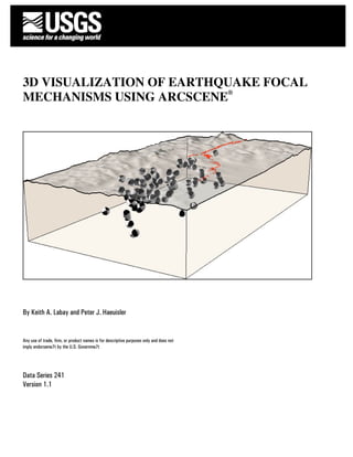
17. 3.0 Example
Figure 16 shows an example image of focal mechanism symbols created by 3D Focal Mechanisms near the epicenter of
the M7.9 2002 Denali Fault earthquake. View is to the northeast. The junction between the Susitna Glacier Thrust Fault and
Denali Fault is shown. Note numerous thrust focal mechanism symbols in the region between the surface rupture of the
Denali Fault and the arc of the Susitna Glacier Thrust Fault. Additional information in this image showing the land surface,
fault location, and the block diagram was added in ArcScene® independent of 3DFM.
Figure 16. Example image of focal mechanism symbols along the Denali Fault and Susitna Glacier Thrust Fault.
4.0 References Cited
Brune, J.N., 1970, Tectonic stress and the spectra of seismic shear waves from earthquakes: Journal
of Geophysical Research, v. 75, no. 26, p. 4997-5009.
Cronin, V.S., 2004, A draft primer on focal mechanism solutions for geologists: Teaching Quantita-
tive Skills in the Geosciences,
http://serc.carleton.edu/files/NAGTWorkshops/structure04/Focal_mechanism_primer.pdf (last
accessed November 15, 2006).
5.0 Acknowledgments
The authors gratefully acknowledge comments on this text and software functionally from Evan Thoms, Luke Blair,
Bill Ellsworth, and Stephanie Prejean.
17