
Recomendados
Recomendados
Mais conteúdo relacionado
Mais procurados
Mais procurados (20)
Destaque
Destaque (20)
Semelhante a TikZ for economists
Semelhante a TikZ for economists (20)
Último
Último (20)
TikZ for economists
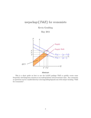
- 1. usepackage{TikZ } for economists Kevin Goulding May 2011 P q ¯ Supply Supply Shift pe B A p∗ 1 p P (q) = − 2 q + 5.25 C Pc P (q) = − 2 q + 9 1 2 ∆T S Q q∗ qe q Abstract This is a short guide on how to use the LaTeX package TikZ to quickly create some frequently used diagrams common to an undergraduate microeconomics class. Any comments or questions can be e-mailed directly to kevingoulding@gmail.com with subject heading “TikZ for economists”. 1
- 2. Introduction TikZ is a package that is useful for creating graphics by via coding direclty in your LaTek document. For example, rather than generating a graphic file (.pdf, .jpg, etc.) and linking to it in your LaTeX code, you include TikZ code in your LaTeX document that tells your compiler how to draw. There are several advantages to using TikZ code: 1. Less complicated file structure - all your figures are self-contained within your LaTeX doc- ument. 2. Beautiful results, with no loss of resolution when scaled up or down. 3. The ability to change diagrams by referencing variables within TikZ code. Header At the very top of you LaTeX document, always include: 1 usepackage { t i k z } And, when you would like to begin a new TikZ diagram within your document, start (and finish it) with this code: 1 begin { t i k z p i c t u r e } % e n t e r TikZ code h e r e . 3 end{ t i k z p i c t u r e } A simple example In this section, we will walk through the creation of the picture in Figure 1 at a high level, just to let you know in broad terms what is going on in the code shown below. Starting the Figure The first line of code (3) tells LaTeX to interpret the following code using the TikZ compiler. Here you also specify the scale of your image. This image has a scale value of 1.1, representing a 10% size increase over no scaling. Line 4 invokes a TikZ packages that allows you to calculate relative coordinate positions (see line 15 for an example of this). 2
- 3. Defining Coordinates Lines 7-11 define the coordinates we will be using in this image as well as the specific labels we would like to place next to the coordinates. For example, line 8 says to define a coordinate A located at the cartesian coordinates (-2.5,2.5) and label the coordinate with a letter “A” above the coordinate. Later in the code we will be able to reference this coordinate simply as “A”. Notice that all the coordinate labels are surrounded by $, thus invoking LaTeX’s math-mode. All code in math-mode (from the amsmath package) works here for labelling. Figure 1: A two-node network electricity A B GA ⇒ cheap K GB ⇒ dear 1 % TikZ code : F i g u r e 1 : A two−node network 3 b e g i n { t i k z p i c t u r e } [ s c a l e =1.1 , t h i c k ] u s e t i k z l i b r a r y { c a l c } %a l l o w s c o o r d i n a t e c a l c u l a t i o n s . 5 % Define coordinates . 7 coordinate [ l a b e l= above : $A$ ] (A) a t ( − 2 . 5 , 2 . 5 ) ; coordinate [ l a b e l= above : $B$ ] (B) a t ( 2 . 5 , 2 . 5 ) ; 9 coordinate [ l a b e l= above : $ e l e c t r i c i t y $ ] (C) a t ( 0 , 3 . 2 5 ) ; coordinate [ l a b e l= above : $G A Rightarrow cheap $ ] (D) a t ( − 3 , 1 . 5 ) ; 11 coordinate [ l a b e l= above : $G B Rightarrow d e a r $ ] (E) a t ( 3 , 1 . 5 ) ; 13 % Draw l i n e s and arrows . draw (A) −− (B) ; 15 draw[−>] ( $ (A) + ( 1 , 0 . 7 5 ) $ ) −− ( $ (B) +( −1 ,0.75) $ ) ; draw [ d e n s e l y d o t t e d ] ( 0 , 2 . 8 ) −− ( 0 , 2 . 2 ) node [ below ] {$K$ } ; 17 draw [ d e n s e l y d o t t e d ] ( 0 . 0 5 , 2 . 8 ) −− ( 0 . 0 5 , 2 . 2 ) ; 19 % Color i n c o o r d i n a t e s . f i l l [ p u r p l e ] (A) c i r c l e ( 3 pt ) ; 21 f i l l [ p u r p l e ] (B) c i r c l e ( 3 pt ) ; 23 end{ t i k z p i c t u r e } Drawing lines and arrows Lines 14-17 essentially connects the coordinates with lines. Line 14 draws a line from coordinate A to coordinate B (as defined above). Line 15 calculates two new coordinates relative to coordinates 3
- 4. A and B, and connects them with an arrowed line by using the command [–¿]. The ability to calculate new coordinates in positions relative to other coordinates is a handy feature available in TikZ. For example, line 15 draws an (arrowed) line from a coordinate 1 unit to the right of coordinate A and 0.75 units above coordinate A to a new coordinate one unit to the left of coordinate B and 0.75 units above. Notice that these relative coordinate calculations need to be enclosed in $. Lines 16 and 17 draw the small vertical lines above “K” in the diagram. Calling “densely dotted” changes the look of the line. Other types of lines are “dotted”, “dashed”, “thick” and several others. Because we called “thick” in line 4 of code, all these lines are a bit thicker than if we had not called the command. You can delete the option “thick” and do a visual comparison. Coloring Coordinates Lines 20 & 21 add the little note of color that you see in our diagram – the nodes in our network (coordinates A and B) are both small circles filled in with the color purple. This is accomplished with the “file” command. Note that colors other than purple can be invoked; feel free to try any of the usual colors (e.g. “green”, “blue”, “orange”, etc.). The command circle draws a circle around coordinate A or B, and “(3pt)” determines the size of the circle. A Few Things to Notice TikZ code differs from LaTeX code in several ways: 1. In TikZ, each line must end in a semicolon. 2. Locations are specified via Cartesian Coordinates. Where is the origin? → The origin is horizontally centered on the page, but its vertical placement depends on the size of the entire picture. Ideally, the simple example shown above will give you an idea of how far a one-unit change represents. For example, the horizontal distance between node A and node B in Figure 1 is 5 units. 3. Similar to LaTeX code, most functions begin with a backward slash. Defining Parameters TikZ allows you to define parameter values and subsequently reference those values throughout your image (or the entire LaTeX) document. This feature enables you to update images quicker once you’ve set up your images as manipulations of parameters. The following is the TikZ code to define a parameter “inc” and set its value to 50. 1 def i n c {50} 4
- 5. You will now be able to reference “inc” elsewhere in your figure. For example, the following code defines two parameters, then uses those parameter values to define a coordinate. In this case, x2 will be located at (0, inc ). pb 1 %D e f i n e p a r a m e t e r s def i n c {50} % parameter i n c s e t = 50 3 def pa { 1 9 . 5 } % parameter pa s e t = 1 9 . 5 5 % Define coordinates . coordinate ( x 2 ) a t ( 0 , { i n c /pb } ) ; Plotting functions TikZ allows you to plot functions. For example, see the following code. draw [ domain = 0 . 6 : 6 ] p l o t ( x , { 1 0 ∗ exp (−1∗x −0.2) +0.3}) ; The code above plots the following function: f (x) = 10e−x−0.2 + 0.3 where x ∈ [0.6, 6] For the most part, functions can be specified using intuitive notation. For best results, install gnuplot on your computer, and you can access a larger set of functions. See http://www.texample.net/tikz/examples/tag/gnuplot/ for more of the capabilities of TikZ coupled with gnuplot. The following example adds axes and a grid using the ‘grid’ specification with the ‘draw’ function. f (x) f (x) = 0.5x x 5
- 6. 1 b e g i n { t i k z p i c t u r e } [ domain = 0 : 4 ] 3 % Draw g r i d l i n e s . draw [ v e r y t h i n , c o l o r=gray ] ( −0.1 , −1.1) g r i d ( 3 . 9 , 3 . 9 ) ; 5 % Draw x and f ( x ) a x e s . 7 draw[−>] ( − 0 . 2 , 0 ) −− ( 4 . 2 , 0 ) node [ r i g h t ] {$ x $ } ; draw[−>] ( 0 , − 1 . 2 ) −− ( 0 , 4 . 2 ) node [ above ] {$ f ( x ) $ } ; 9 % P l o t l i n e w i t h s l o p e = 1/2 , i n t e r c e p t = 1 . 5 11 draw [ c o l o r=b l u e ] p l o t ( x , { 1 . 5 + 0 . 5 ∗ x } ) node [ r i g h t ] {$ f ( x ) = 0 . 5 x $ } ; 13 end{ t i k z p i c t u r e } Coloring Area TikZ is capable of shading in areas of your diagram, bounded by coordinate or functions. This can be achieved by calling the ‘fill’ function as in the following example: f i l l [ o r a n g e ! 6 0 ] ( 0 , 0 ) −− ( 0 , 1 ) −− ( 1 , 1 ) −− ( 1 , 0 ) −− c y c l e ; This colors in a 1x1 square with orange (at 60% opacity). Basically, it will connect the listed coordinates with straight lines creating an outline that will be shaded in by the chosen color. Note the command ‘cycle’ at the end. This closes the loop by connecting the last listed coordinate back to the first. You can also bound the area to be shaded by a non-straight line. The following example shades in the area under a normal distribution bounded by 0 and 4.4: 1 % d e f i n e normal d i s t r i b u t i o n f u n c t i o n ’ normaltwo ’ def normaltwo {x , { 4 ∗ 1 / exp ( ( ( x−3) ˆ 2 ) / 2 ) }} 3 5 % Shade orange are a u n d e r n e a t h c u r v e . f i l l [ f i l l =o r a n g e ! 6 0 ] ( 2 . 6 , 0 ) −− p l o t [ domain = 0 : 4 . 4 ] ( normaltwo ) −− ( 4 . 4 , 0 ) −− cycle ; 7 % Draw and l a b e l normal d i s t r i b u t i o n f u n c t i o n 9 draw [ dashed , c o l o r=blue , domain = 0 : 6 ] p l o t ( normaltwo ) node [ r i g h t ] {$N( mu, sigma ˆ 2 ) $}; 6
- 7. N (µ, σ 2 ) And, here is another example that includes axes and two interior bounds on the shading: 1 begin { t i k z p i c t u r e } % d e f i n e normal d i s t r i b u t i o n f u n c t i o n ’ normaltwo ’ 3 def normaltwo {x , { 4 ∗ 1 / exp ( ( ( x−3) ˆ 2 ) / 2 ) }} 5 % i n p u t x and y p a r a m e t e r s def y { 4 . 4 } 7 def x { 3 . 4 } 9 % this line calculates f (y) def f y {4∗1/ exp ( ( ( y−3) ˆ 2 ) / 2 ) } 11 def f x {4∗1/ exp ( ( ( x−3) ˆ 2 ) / 2 ) } 13 % Shade orange are a u n d e r n e a t h c u r v e . f i l l [ f i l l =o r a n g e ! 6 0 ] ( { x } , 0 ) −− p l o t [ domain={x } : { y } ] ( normaltwo ) −− ( { y } , 0 ) −− c y c l e ; 15 % Draw and l a b e l normal d i s t r i b u t i o n f u n c t i o n 17 draw [ c o l o r=blue , domain = 0 : 6 ] p l o t ( normaltwo ) node [ r i g h t ] { } ; 19 % Add dashed l i n e d r o p p i n g down from normal . draw [ dashed ] ( { y } , { f y } ) −− ( { y } , 0 ) node [ below ] {$ y $ } ; 21 draw [ dashed ] ( { x } , { f x } ) −− ( { x } , 0 ) node [ below ] {$ x $ } ; 23 % O p t i o n a l : Add a x i s l a b e l s draw ( − . 2 , 2 . 5 ) node [ l e f t ] {$ f Y( u ) $ } ; 25 draw ( 3 , − . 5 ) node [ below ] {$u $ } ; 27 % O p t i o n a l : Add a x e s draw[−>] ( 0 , 0 ) −− ( 6 . 2 , 0 ) node [ r i g h t ] { } ; 29 draw[−>] ( 0 , 0 ) −− ( 0 , 5 ) node [ above ] { } ; 31 end{ t i k z p i c t u r e } 7
- 8. fY (u) x y u Some TikZ diagrams with code The following diagrams were done in TikZ. Budget Constraints and Indifference Curves Figure 2: A Generic Price Change x2 M p2 IC2 IC1 x1 1 % TikZ code : F i g u r e 2 : A Generic P r i c e Change 3 b e g i n { t i k z p i c t u r e } [ domain =0:5 , r a n g e =4:5 , s c a l e =1, t h i c k ] u s e t i k z l i b r a r y { c a l c } %a l l 5 %D e f i n e l i n e a r p a r a m e t e r s f o r s u p p l y and demand 8
- 9. 7 def i n c {50} %Enter t o t a l income def pa { 1 9 . 5 } %P r i c e o f x 1 9 def pb {10} %P r i c e o f x 2 . def panew { 1 0 . 6 } 11 def i c a {x , { 1 0 / x }} 13 def i c b {x , { s s l p ∗ x+ s i n t }} def demandtwo {x , { d s l p ∗ x+d i n t+dsh }} 15 def supplytwo {x , { s s l p ∗ x+ s i n t +s s h }} 17 % Define coordinates . 19 coordinate ( x 2 ) a t ( 0 , { i n c /pb } ) ; coordinate ( x 1 ) a t ( { i n c / pa } , 0 ) ; 21 coordinate ( x 1 ’ ) a t ( { i n c / panew } , 0 ) ; 23 %Draw axes , and d o t t e d e q u i l i b r i u m l i n e s . draw[−>] ( 0 , 0 ) −− ( 6 . 2 , 0 ) node [ r i g h t ] {$ x 1 $ } ; 25 draw[−>] ( 0 , 0 ) −− ( 0 , 6 . 2 ) node [ above ] {$ x 2 $ } ; draw [ t h i c k ] ( x 1 ) −− ( x 2 ) node [ l e f t ] {$ f r a c {M}{p 2 } $ } ; 27 draw [ t h i c k ] ( x 1 ’ ) −− ( x 2 ) ; draw [ t h i c k , c o l o r=p u r p l e , domain = 0 . 6 : 6 ] p l o t ( x , { 1 0 ∗ exp (−1∗x −0.2) +0.3}) node [ r i g h t ] {IC $ 1 $ } ; 29 draw [ t h i c k , c o l o r=p u r p l e , domain = 1 : 6 ] p l o t ( x , { 1 0 ∗ exp ( −0.8∗ x ) +1}) node [ r i g h t ] {IC $ 2 $ } ; 31 draw [ d o t t e d ] ( 1 . 5 , 2 ) −− ( 1 . 5 , 0 ) ; draw [ d o t t e d ] ( 2 . 5 , 2 . 3 5 ) −− ( 2 . 5 , 0 ) ; 33 end{ t i k z p i c t u r e } % TikZ code : F i g u r e 3 : A Budget c o n s t r a i n t t h a t has a voucher f o r x 1 2 b e g i n { t i k z p i c t u r e } [ domain =0:5 , r a n g e =4:5 , s c a l e =1, t h i c k ] u s e t i k z l i b r a r y { c a l c } %a l l 4 %D e f i n e l i n e a r p a r a m e t e r s f o r s u p p l y and demand 6 def i n c {62} %Enter t o t a l income def pa { 1 9 . 5 } %P r i c e o f x 1 8 def pb {10} %P r i c e o f x 2 . def panew { 1 0 . 6 } 10 def i c a {x , { 2 / x−20}} 12 def i c b {x , { s s l p ∗ x+ s i n t }} 14 def bcv {x ,{( − pa ) / ( pb ) ∗ x+( i n c ) / ( pb ) }} 9
- 10. Figure 3: A Budget constraint that has a voucher for x1 x2 voucher Indiff. Curve x1 Budget Constraint def bcx {x , { ( 5 ) / x }} 16 % Define coordinates . 18 coordinate ( x 2 ) a t ( 0 , { i n c /pb } ) ; coordinate ( x 1 ) a t ( { i n c / pa } , 0 ) ; 20 coordinate ( x 1 ’ ) a t ( { i n c / panew } , 0 ) ; 22 %Draw axes , and d o t t e d e q u i l i b r i u m l i n e s . draw[−>] ( 0 , 0 ) −− ( 6 . 2 , 0 ) node [ r i g h t ] {$ x 1 $ } ; 24 draw[−>] ( 0 , 0 ) −− ( 0 , 6 . 2 ) node [ above ] {$ x 2 $ } ; draw [ dashed ] ( 1 . 2 , 3 . 9 ) −− ( 0 , 3 . 9 ) node [ l e f t ] { voucher } ; 26 draw [ t h i c k , domain = 1 . 2 : i n c / pa ] p l o t ( bcv ) node [ below ] { Budget C o n s t r a i n t } ; draw [ t h i c k , c o l o r=p u r p l e , domain = 1 : 5 ] p l o t ( bcx ) node [ below ] { I n d i f f . Curve } ; 28 end{ t i k z p i c t u r e } 10
- 11. Income & Substitution Effects Figure 4: A decrease in the price of x1 by one-fourth x2 M BC2 p2 BC1 e∗ 2 e∗ 1 e1 IC2 IC1 x1 Substitution Effect Income Effect Total Effect 1 % TikZ code : F i g u r e 4 : A d e c r e a s e i n t h e p r i c e o f x 1 by one−f o u r t h 3 b e g i n { t i k z p i c t u r e } [ domain =0:100 , r a n g e =0:200 , s c a l e =0.4 , t h i c k , f o n t = s c r i p t s i z e ] u s e t i k z l i b r a r y { c a l c } %a l l 5 %D e f i n e l i n e a r p a r a m e t e r s f o r s u p p l y and demand 7 def i n c {10} %Enter t o t a l income def pa {1} %P r i c e o f x 1 9 def pb {1} %P r i c e o f x 2 . def panew { 0 . 2 5 } 11 % d e f i c a { x , { 1 0 / x }} 13 % d e f i c b { x , { s s l p ∗ x+ s i n t }} % d e f demandtwo { x , { d s l p ∗ x+ d i n t +dsh }} 15 % d e f s u p p l y t w o { x , { s s l p ∗ x+ s i n t +s s h }} 17 % Define coordinates . 19 coordinate ( x 2 ) a t ( 0 , { i n c /pb } ) ; coordinate ( x 1 ) a t ( { i n c / pa } , 0 ) ; 21 coordinate ( x 1 ’ ) a t ( { i n c / panew } , 0 ) ; 23 coordinate [ l a b e l= r i g h t : $ e ˆ ∗ 1 $ ] ( p 1 ) a t ( 5 , 5 ) ; coordinate [ l a b e l= above : $ e 1 ’ $ ] ( p 2 ) a t ( 1 0 , 2 . 5 ) ; 25 coordinate [ l a b e l= above : $ e ˆ ∗ 2 $ ] ( p 3 ) a t ( 2 0 , 5 ) ; 27 %Draw axes , and d o t t e d e q u i l i b r i u m l i n e s . 11
- 12. draw[−>] ( 0 , 0 ) −− ( 4 2 , 0 ) node [ r i g h t ] {$ x 1 $ } ; 29 draw[−>] ( 0 , 0 ) −− ( 0 , 1 2 ) node [ above ] {$ x 2 $ } ; draw [ t h i c k ] ( x 1 ) −− ( x 2 ) node [ l e f t ] {$ f r a c {M}{p 2 } $ } ; 31 draw [ t h i c k ] ( x 1 ’ ) −− ( x 2 ) ; % draw [ t h i c k , c o l o r=p u r p l e , domain = 0 . 6 : 1 0 0 ] p l o t ( x , { 1 5 ∗ exp ( x ) }) node [ r i g h t ] {IC $ 1 $ } ; 33 % draw [ t h i c k , c o l o r=p u r p l e , domain = 0 . 6 : 1 0 0 ] p l o t f u n c t i o n ( x , { ( 2 5 0 0 ) /( x ) }) node [ r i g h t ] {IC $ 1 $ } ; draw [ t h i c k , c o l o r=green , domain = 2 : 2 5 ] p l o t ( x , { ( 2 5 ) / ( x ) } ) node [ r i g h t ] {IC $ 1$}; 35 draw [ t h i c k , c o l o r=green , domain = 8 : 3 0 ] p l o t ( x , { ( 1 0 0 ) / ( x ) } ) node [ r i g h t ] {IC $ 2$}; 37 draw ( 2 , 8 ) node [ l a b e l= below : $BC 1 $ ] { } ; draw ( 5 , 1 1 . 5 ) node [ l a b e l= below : $BC 2 $ ] { } ; 39 draw [ d o t t e d ] ( p 2 ) −− ( 1 0 , 0 ) ; 41 draw [ d o t t e d ] ( p 1 ) −− ( 5 , 0 ) ; draw [ d o t t e d ] ( p 3 ) −− ( 2 0 , 0 ) ; 43 draw [ dashed ] ( 0 , 5 ) −− ( 2 0 , 0 ) ; 45 draw[<−] ( 9 . 8 , − 1 ) −− (5 , −1) node [ l e f t ] { S u b s t i t u t i o n E f f e c t } ; 47 draw[−>] (10 , −1) −− (20 , −1) node [ r i g h t ] { Income E f f e c t } ; draw[−>, d e n s e l y dashed ] (5 , −2) −− (20 , −2) ; 49 draw ( 1 2 . 5 , − 2 ) node [ l a b e l= below : T o t a l E f f e c t ] { } ; 51 f i l l [ b l u e ] ( p 1 ) c i r c l e ( 6 pt ) ; f i l l [ b l u e ] ( p 2 ) c i r c l e ( 6 pt ) ; 53 f i l l [ b l u e ] ( p 3 ) c i r c l e ( 6 pt ) ; 55 end{ t i k z p i c t u r e } 1 % TikZ code : F i g u r e 5 : A d e c r e a s e i n t h e p r i c e o f x 1 by half . 3 b e g i n { t i k z p i c t u r e } [ domain =0:100 , r a n g e =0:200 , s c a l e =0.7 , t h i c k ] usetikzlibrary { calc } 5 %D e f i n e l i n e a r p a r a m e t e r s f o r s u p p l y and demand 7 def i n c {10} %Enter t o t a l income def pa {1} %P r i c e o f x 1 9 def pb {1} %P r i c e o f x 2 . def panew { 0 . 5 } %New p r i c e f o r x 1 . 11 % Define coordinates . 13 coordinate ( x 2 ) a t ( 0 , { i n c /pb } ) ; coordinate ( x 1 ) a t ( { i n c / pa } , 0 ) ; 15 coordinate ( x 1 ’ ) a t ( { i n c / panew } , 0 ) ; 12
- 13. Figure 5: A decrease in the price of x1 by half. x2 M p2 BC2 BC1 e∗ 2 e∗ 1 e1 IC2 IC1 x1 Substitution Effect Income Effect Total Effect 17 coordinate [ l a b e l= r i g h t : $ e ˆ ∗ 1 $ ] ( p 1 ) a t ( 5 , 5 ) ; coordinate [ l a b e l= above : $ e 1 ’ $ ] ( p 2 ) a t ( 7 . 0 7 , 3 . 5 3 ) ; 19 coordinate [ l a b e l= above : $ e ˆ ∗ 2 $ ] ( p 3 ) a t ( 1 0 , 5 ) ; 21 %Draw axes , and d o t t e d e q u i l i b r i u m l i n e s . draw[−>] ( 0 , 0 ) −− ( 2 0 . 5 , 0 ) node [ r i g h t ] {$ x 1 $ } ; 23 draw[−>] ( 0 , 0 ) −− ( 0 , 1 2 ) node [ above ] {$ x 2 $ } ; draw [ t h i c k ] ( x 1 ) −− ( x 2 ) node [ l e f t ] {$ f r a c {M}{p 2 } $ } ; 25 draw [ t h i c k ] ( x 1 ’ ) −− ( x 2 ) ; 27 %Draw i n d i f f e r e n c e c u r v e s draw [ t h i c k , c o l o r=green , domain = 2 : 1 8 ] p l o t ( x , { ( 2 5 ) / ( x ) } ) node [ r i g h t ] {IC $ 1$}; 29 draw [ t h i c k , c o l o r=green , domain = 3 . 9 : 1 8 ] p l o t ( x , { ( 5 0 ) / ( x ) } ) node [ r i g h t ] {IC $ 2$}; 31 %L a b e l b u d g e t c o n s t r a i n t draw ( 2 , 7 . 8 ) node [ l a b e l= below : $BC 1 $ ] { } ; 33 draw ( 4 . 5 , 9 . 1 ) node [ l a b e l= below : $BC 2 $ ] { } ; 13
- 14. 35 %Draw d o t t e d l i n e s showing quantities . draw [ d o t t e d ] ( p 2 ) −− (7.07 ,0) ; 37 draw [ d o t t e d ] ( p 1 ) −− (5 ,0) ; draw [ d o t t e d ] ( p 3 ) −− (10 ,0) ; 39 %L a b e l S u b s t i t u t i o n , Income , and T o t a l e f f e c t s . 41 draw [ dashed ] ( 0 , 7 . 0 7 ) −− ( 1 4 . 1 4 , 0 ) ; draw[<−] (7 , −1) −− (5 , −1) node [ l e f t ] { S u b s t i t u t i o n E f f e c t } ; 43 draw[−>] ( 7 . 0 7 , − 1 ) −− (10 , −1) node [ r i g h t ] { Income E f f e c t } ; draw[−>, d e n s e l y dashed ] (5 , −2) −− (10 , −2) ; 45 draw ( 7 . 5 , − 2 ) node [ l a b e l= below : T o t a l E f f e c t ] { } ; 47 %C r e a t e p o i n t s where IC t a n g e n t i a l l y i n t e r s e c t s t h e b u d g e t c o n s t r a i n t . f i l l [ b l u e ] ( p 1 ) c i r c l e ( 4 pt ) ; 49 f i l l [ b l u e ] ( p 2 ) c i r c l e ( 4 pt ) ; f i l l [ b l u e ] ( p 3 ) c i r c l e ( 4 pt ) ; 51 f i l l [ b l u e ] ( 7 . 0 7 , 3 . 5 3 ) c i r c l e ( 4 pt ) ; 53 end{ t i k z p i c t u r e } % TikZ code : F i g u r e XX: A two−node network Some Useful Diagrams Figure 6: A piecewise-defined electricity bid $ MW MW % TikZ code : F i g u r e 6 : A p i e c e w i s e −d e f i n e d e l e c t r i c i t y b i d 2 b e g i n { t i k z p i c t u r e } [ domain =0:5 , s c a l e =1, t h i c k ] 4 14
- 15. %D e f i n e b i d q u a n t i t i e s 6 def qone {3} % step 1 def qtwo {2} % step 2 8 def q t h r e e {1} % step 3 def q f o u r { 0 . 5 } % step 4 10 %D e f i n e b i d p r i c e s 12 def pone {1} % step 1 def ptwo {2} % step 2 14 def p t h r e e {4} % step 3 def p f o u r { 5 . 5 } % step 4 16 18 % Define coordinates . 20 coordinate ( l o n e ) a t ( 0 , { pone } ) ; coordinate ( l t w o ) a t ( { qone } , { ptwo } ) ; 22 coordinate ( l t h r e e ) a t ( { qtwo+qone } , { p t h r e e } ) ; coordinate ( l f o u r ) a t ( { q t h r e e+qtwo+qone } , { p f o u r } ) ; 24 coordinate ( r o n e ) a t ( { qone } , { pone } ) ; 26 coordinate ( rtwo ) a t ( { qtwo+qone } , { ptwo } ) ; coordinate ( r t h r e e ) a t ( { q t h r e e+qtwo+qone } , { p t h r e e } ) ; 28 coordinate ( r f o u r ) a t ( { q f o u r+q t h r e e+qtwo+qone } , { p f o u r } ) ; 30 coordinate ( done ) a t ( { qone } , 0 ) ; coordinate ( dtwo ) a t ( { qtwo+qone } , 0 ) ; 32 coordinate ( d t h r e e ) a t ( { q t h r e e+qtwo+qone } , 0 ) ; coordinate ( d f o u r ) a t ( { q f o u r+q t h r e e+qtwo+qone } , 0 ) ; 34 %Draw a x e s 36 draw[−>] ( 0 , 0 ) −− ( 6 . 2 , 0 ) node [ r i g h t ] {$M } ; W$ draw[−>] ( 0 , 0 ) −− ( 0 , 6 . 2 ) node [ l e f t ] {$ f r a c {$}{M $ } ; W} 38 %Draw b i d s t e p s 40 draw [ t h i c k , c o l o r=b l u e ] ( l o n e ) −− ( r o n e ) ; draw [ t h i c k , c o l o r=b l u e ] ( l t w o ) −− ( rtwo ) ; 42 draw [ t h i c k , c o l o r=b l u e ] ( l t h r e e ) −− ( r t h r e e ) ; draw [ t h i c k , c o l o r=b l u e ] ( l f o u r ) −− ( r f o u r ) ; 44 %Draw dashed l i n e s 46 draw [ dashed ] ( l t w o ) −− ( r o n e ) ; draw [ dashed ] ( l t h r e e ) −− ( rtwo ) ; 48 draw [ dashed ] ( l f o u r ) −− ( r t h r e e ) ; 50 end{ t i k z p i c t u r e } 1 % TikZ code : F i g u r e 7 : The area b e t w e e n two c u r v e s 15
- 16. Figure 7: The area between two curves f (ˆ) x +φ −φ λ2 λ1 µ2 x ˆ 64th 3 b e g i n { t i k z p i c t u r e } [ s c a l e =2] %f o n t = s c r i p t s i z e ] 5 %Note : 64 t h p e r c e n t i l e i s 0 . 3 6 s t a n d a r d d e v i a t i o n s t o t h e r i g h t o f mean . 7 %D e f i n e e q u a t i o n s f o r t h e two normal d i s t r i b u t i o n s . def normalone {x , { 4 ∗ 1 / exp ( ( ( x−4) ˆ 2 ) / 2 ) }} 9 def normaltwo {x , { 4 ∗ 1 / exp ( ( ( x−3) ˆ 2 ) / 2 ) }} 11 %Shade orange are a f i l l [ f i l l =o r a n g e ! 6 0 ] ( 2 . 6 , 0 ) −− p l o t [ domain = 2 . 6 : 3 . 4 ] ( normaltwo ) −− ( 3 . 4 , 0 ) −− c y c l e ; 13 f i l l [ f i l l =w h i t e ] ( 2 . 6 , 0 ) −− p l o t [ domain = 2 . 6 : 3 . 4 ] ( normalone ) −− ( 3 . 4 , 0 ) −− cycle ; 15 %Draw b l u e normal d i s t r i b u t i o n s 16
- 17. draw [ t h i c k , c o l o r=blue , domain = 0 : 6 ] p l o t ( normalone ) node [ r i g h t ] {$lambda 1 $ } ; 17 draw [ t h i c k , c o l o r=blue , domain = 0 : 5 ] p l o t ( normaltwo ) node [ r i g h t ] {$lambda 2 $ } ; 19 %Draw a x e s draw[−>] ( 0 , 0 ) −− ( 6 . 2 , 0 ) node [ r i g h t ] {$ hat{x } $ } ; 21 draw[−>] ( 0 , 0 ) −− ( 0 , 6 . 2 ) node [ l e f t ] {$ f ( hat{x } ) $ } ; 23 %D e f i n e c o o r d i n a t e s coordinate ( muone ) a t (4 ,4) ; 25 coordinate ( mutwo ) a t (3 ,4) ; 27 %Draw dashed l i n e s from mean t o x−a x i s draw [ dashed ] ( muone ) −− ( 4 , 0 ) node [ below ] {$64ˆ{ th } $ } ; 29 draw [ dashed ] ( mutwo ) −− ( 3 , 0 ) node [ below ] {$mu 2 $ } ; 31 draw [ dashed ] ( 2 . 6 , 0 ) −− p l o t [ domain = 2 . 5 9 : 2 . 6 ] ( normaltwo ) node [ l e f t ] {$−phi $}; draw [ dashed ] ( 3 . 4 , 0 ) −− p l o t [ domain = 3 . 3 9 : 3 . 4 ] ( normaltwo ) node [ above ] {$+phi $}; 33 35 end{ t i k z p i c t u r e } Game Theory Diagrams See below, customizable diagrams for mapping strategic games. Figure 8: A 2×2 Strategic form game Firm B Left Right 57 54 Top 57 72 Firm A 72 64 Bot 54 64 1 % TikZ code : F i g u r e 8 : A 2 x 2 S t r a t e g i c form game 3 b e g i n { t i k z p i c t u r e } [ s c a l e =2] %f o n t = s c r i p t s i z e ] 17
- 18. 5 % O u t l i n e box draw [ t h i c k ] ( 0 , 0 ) −− ( 2 . 2 , 0 ) ; 7 draw [ t h i c k ] ( 0 , 0 ) −− ( 0 , 2 . 2 ) ; draw [ t h i c k ] ( 2 . 2 , 2 . 2 ) −− ( 2 . 2 , 0 ) ; 9 draw [ t h i c k ] ( 2 . 2 , 2 . 2 ) −− ( 0 , 2 . 2 ) ; draw [ t h i c k ] ( − 0 . 3 , 1 . 1 ) −− ( 2 . 2 , 1 . 1 ) ; 11 draw [ t h i c k ] ( 1 . 1 , 0 ) −− ( 1 . 1 , 2 . 5 ) ; 13 % Payoff d i v i d e r s draw [ d e n s e l y d o t t e d ] ( . 1 , 2 . 1 ) −− ( 1 , 1 . 2 ) ; 15 draw [ d e n s e l y d o t t e d ] ( . 1 , 1 ) −− ( 1 , 0 . 1 ) ; draw [ d e n s e l y d o t t e d ] ( 1 . 2 , 1 ) −− ( 2 . 1 , 0 . 1 ) ; 17 draw [ d e n s e l y d o t t e d ] ( 1 . 2 , 2 . 1 ) −− ( 2 . 1 , 1 . 2 ) ; 19 % Strategy lab el s coordinate [ l a b e l= l e f t : Top ] ( p 1 ) a t ( −0.1 ,1.6) ; 21 coordinate [ l a b e l= l e f t : Bot ] ( p 1 ) a t ( −0.1 ,0.4) ; 23 coordinate [ l a b e l= above : L e f t ] ( p 1 ) a t ( 0 . 5 5 , 2 . 2 ) ; coordinate [ l a b e l= above : Right ] ( p 1 ) a t ( 1 . 6 5 , 2 . 2 ) ; 25 coordinate [ l a b e l= above : bf {Firm B} ] ( p 1 ) a t ( 1 . 1 , 2 . 5 ) ; 27 coordinate [ l a b e l= l e f t : bf {Firm A} ] ( p 1 ) a t ( − 0 . 3 , 1 . 1 ) ; 29 % The p a y o f f s f o r b o t h p l a y e r s : 31 f i l l [ red ] ( . 3 5 , 1 . 4 ) node { $ 5 7 $ } ; f i l l [ blue ] ( 0 . 8 , 1 . 9 ) node { $ 5 7 $ } ; 33 f i l l [ red ] ( 1 . 4 , 1 . 4 ) node { $ 7 2 $ } ; 35 f i l l [ blue ] ( 1 . 9 , 1 . 9 ) node { $ 5 4 $ } ; 37 f i l l [ red ] ( 0 . 3 5 , 0 . 3 5 ) node { $ 5 4 $ } ; f i l l [ blue ] ( 0 . 8 , 0 . 8 ) node { $ 7 2 $ } ; 39 f i l l [ red ] ( 1 . 4 , 0 . 3 5 ) node { $ 6 4 $ } ; 41 f i l l [ blue ] ( 1 . 9 , 0 . 8 ) node { $ 6 4 $ } ; 43 end{ t i k z p i c t u r e } % TikZ code : F i g u r e XX: A 3 x 3 S t r a t e g i c form game 2 b e g i n { t i k z p i c t u r e } [ s c a l e =2] 4 % Outline matrix 6 draw [ t h i c k ] ( 0 , 0 ) −− (3.3 ,0) ; draw [ t h i c k ] ( 0 , 0 ) −− (0 ,3.3) ; 8 draw [ t h i c k ] (3.3 ,3.3) −− ( 3 . 3 , 0 ) ; draw [ t h i c k ] (3.3 ,3.3) −− ( 0 , 3 . 3 ) ; 18
- 19. Figure 9: A 3×3 Strategic form game Firm B Left Middle Right 64 64 64 Top 64 64 64 57 54 64 Firm A Mid 57 72 64 72 64 64 Bot 54 64 64 10 draw [ t h i c k ] ( −0.3 ,1.1) −− ( 3 . 3 , 1 . 1 ) ; draw [ t h i c k ] ( −0.3 ,2.2) −− ( 3 . 3 , 2 . 2 ) ; 12 draw [ t h i c k ] ( 1 . 1 , 0 ) −− (1.1 ,3.6) ; draw [ t h i c k ] ( 2 . 2 , 0 ) −− (2.2 ,3.6) ; 14 draw [ d e n s e l y dotted ] ( . 1 , 2 . 1 ) −− ( 1 , 1 . 2 ) ; 16 draw [ d e n s e l y dotted ] ( . 1 , 1 ) −− ( 1 , 0 . 1 ) ; draw [ d e n s e l y dotted ] ( 1 . 2 , 1 ) −− ( 2 . 1 , 0 . 1 ) ; 18 draw [ d e n s e l y dotted ] ( 1 . 2 , 2 . 1 ) −− ( 2 . 1 , 1 . 2 ) ; 20 draw [ d e n s e l y dotted ] ( . 1 , 3 . 2 ) −− ( 1 , 2 . 3 ) ; draw [ d e n s e l y dotted ] ( 1 . 2 , 3 . 2 ) −− ( 2 . 1 , 2 . 3 ) ; 22 draw [ d e n s e l y dotted ] ( 3 . 2 , . 1 ) −− ( 2 . 3 , 1 ) ; draw [ d e n s e l y dotted ] ( 3 . 2 , 1 . 2 ) −− ( 2 . 3 , 2 . 1 ) ; 24 draw [ d e n s e l y dotted ] ( 3 . 2 , 2 . 3 ) −− ( 2 . 3 , 3 . 2 ) ; 26 coordinate [ l a b e l= r i g h t : Top ] ( p 1 ) a t ( −0.5 ,2.7) ; 28 coordinate [ l a b e l= r i g h t : Mid ] ( p 1 ) a t ( −0.5 ,1.65) ; coordinate [ l a b e l= r i g h t : Bot ] ( p 1 ) a t ( −0.5 ,0.55) ; 30 coordinate [ l a b e l= above : L e f t ] ( p 1 ) a t ( 0 . 5 5 , 3 . 3 ) ; 32 coordinate [ l a b e l= above : Middle ] ( p 1 ) a t ( 1 . 6 5 , 3 . 3 ) ; coordinate [ l a b e l= above : Right ] ( p 1 ) a t ( 2 . 7 , 3 . 3 ) ; 34 coordinate [ l a b e l= above : bf {Firm B} ] ( p 1 ) a t ( 1 . 6 5 , 3 . 7 ) ; 36 coordinate [ l a b e l= l e f t : bf {Firm A} ] ( p 1 ) a t ( − . 8 , 1 . 6 5 ) ; 19
- 20. 38 % F i l l i n pay−o f f s 40 f i l l [ red ] ( . 3 5 , 1 . 4 ) node { $ 5 7 $ } ; %Mid − L e f t f i l l [ blue ] ( 0 . 8 , 1 . 9 ) node { $ 5 7 $ } ; 42 f i l l [ red ] ( 1 . 4 , 1 . 4 ) node { $ 7 2 $ } ; %Mid − Middle 44 f i l l [ blue ] ( 1 . 9 , 1 . 9 ) node { $ 5 4 $ } ; 46 f i l l [ red ] ( 0 . 3 5 , 0 . 3 5 ) node { $ 5 4 $ } ; %Bot − L e f t f i l l [ blue ] ( 0 . 8 , 0 . 8 ) node { $ 7 2 $ } ; 48 f i l l [ red ] ( 1 . 4 , 0 . 3 5 ) node { $ 6 4 $ } ; %Bot − Middle 50 f i l l [ blue ] ( 1 . 9 , 0 . 8 ) node { $ 6 4 $ } ; 52 f i l l [ red ] ( 2 . 5 , 0 . 3 5 ) node { $ 6 4 $ } ; %Bot − R i g h t f i l l [ blue ] ( 3 , 0 . 8 ) node { $ 6 4 $ } ; 54 f i l l [ red ] ( 2 . 5 , 1 . 4 5 ) node { $ 6 4 $ } ; %Mid − R i g h t 56 f i l l [ blue ] ( 3 , 1 . 9 ) node { $ 6 4 $ } ; 58 f i l l [ red ] ( 2 . 5 , 2 . 5 5 ) node { $ 6 4 $ } ; %Top − R i g h t f i l l [ b l u e ] ( 3 , 3 ) node { $ 6 4 $ } ; 60 f i l l [ red ] ( 1 . 4 , 2 . 5 5 ) node { $ 6 4 $ } ; %Top − Middle 62 f i l l [ blue ] ( 1 . 9 , 3 ) node { $ 6 4 $ } ; 64 f i l l [ red ] ( 0 . 3 5 , 2 . 5 5 ) node { $ 6 4 $ } ; %Top − L e f t f i l l [ blue ] ( 0 . 8 , 3 ) node { $ 6 4 $ } ; 66 end{ t i k z p i c t u r e } Figure 10: An Extensive-form game Lef t (57, 57) Firm B Rig h p t To (72, 54) Firm A Bo tto m Lef t (54, 72) Firm B Rig h t (64, 64) 20
- 21. 1 % TikZ code : F i g u r e 1 0 : An E x t e n s i v e −form game 3 % Set the o v e r a l l layout of the t r e e t i k z s t y l e { l e v e l 1}=[ l e v e l d i s t a n c e =3.5cm , s i b l i n g d i s t a n c e =3.5cm ] 5 t i k z s t y l e { l e v e l 2}=[ l e v e l d i s t a n c e =3.5cm , s i b l i n g d i s t a n c e =2cm ] 7 % D e f i n e s t y l e s f o r b a g s and l e a f s t i k z s t y l e { bag } = [ t e x t width=4em , t e x t c e n t e r e d ] 9 t i k z s t y l e { end } = [ c i r c l e , minimum width=3pt , f i l l , i n n e r s e p=0pt ] 11 % The s l o p e d o p t i o n g i v e s r o t a t e d e d g e l a b e l s . P e r s o n a l l y 13 % I f i n d s l o p e d l a b e l s a b i t d i f f i c u l t t o read . Remove t h e s l o p e d o p t i o n s % to get horizontal l a b e l s . 15 b e g i n { t i k z p i c t u r e } [ grow=r i g h t , s l o p e d ] node [ bag ] {Firm A} 17 child { node [ bag ] {Firm B} 19 child { node [ end , l a b e l=r i g h t : 21 { $ ( 6 4 , 6 4 ) $ } ] {} % e n t e r pay−o f f s f o r ( Bottom , R i g h t ) edge from p a r e n t 23 node [ above ] {$ Right $} } 25 child { node [ end , l a b e l=r i g h t : 27 { $ ( 5 4 , 7 2 ) $ } ] {} % e n t e r pay−o f f s f o r ( Bottom , L e f t ) edge from p a r e n t 29 node [ above ] {$ L e f t $} } 31 edge from p a r e n t node [ above ] {$ Bottom $} 33 } child { 35 node [ bag ] {Firm B} child { 37 node [ end , l a b e l=r i g h t : { $ ( 7 2 , 5 4 ) $ } ] {} % e n t e r pay−o f f s f o r ( Top , R i g h t ) 39 edge from p a r e n t node [ above ] {$ Right $} 41 } child { 43 node [ end , l a b e l=r i g h t : { $ ( 5 7 , 5 7 ) $ } ] {} % e n t e r pay−o f f s f o r ( Top , L e f t ) 45 edge from p a r e n t node [ above ] {$ L e f t $} 47 } edge from p a r e n t 49 node [ above ] {$Top$} }; 21
- 22. 51 draw [ r e d ] ( 3 . 5 , 0 ) e l l i p s e ( 1cm and 3cm) ; 53 end{ t i k z p i c t u r e } Taxes, Price ceilings, and market equilibriums Figure 11: An economics example from texample.com E YO A C D B NX = x G ↑ /T ↓ % TikZ code : F i g u r e 1 1 : An economics example from t e x a m p l e . com 2 % −−> See TikZ code i n . t e x f i l e backup or on t e x a m p l e . com . 1 % TikZ code : F i g u r e 1 2 : Market e q u i l i b r i u m − an a l t e r n a t e approach 3 b e g i n { t i k z p i c t u r e } [ s c a l e =3] 5 % Draw a x e s draw [<−>, t h i c k ] ( 0 , 2 ) node ( y a x i s ) [ above ] {$P$} 7 |− ( 3 , 0 ) node ( x a x i s ) [ r i g h t ] {$Q$ } ; 9 % Draw two i n t e r s e c t i n g l i n e s draw ( 0 , 0 ) coordinate ( a 1 ) −− ( 2 , 1 . 8 ) coordinate ( a 2 ) ; 11 draw ( 0 , 1 . 5 ) coordinate ( b 1 ) −− ( 2 . 5 , 0 ) coordinate ( b 2 ) ; 22
- 23. Figure 12: Market equilibrium - an alternate approach P p∗ Q q∗ 13 % C a l c u l a t e t h e i n t e r s e c t i o n o f t h e l i n e s a 1 −− a 2 and b 1 −− b 2 % and s t o r e t h e c o o r d i n a t e i n c . 15 coordinate ( c ) a t ( i n t e r s e c t i o n o f a 1−−a 2 and b 1−−b 2 ) ; 17 % Draw l i n e s i n d i c a t i n g i n t e r s e c t i o n w i t h y and x a x i s . Here we use % t h e p e r p e n d i c u l a r c o o r d i n a t e system 19 draw [ dashed ] ( y a x i s |− c ) node [ l e f t ] {$p ˆ∗$} −| ( x a x i s −| c ) node [ below ] {$ q ˆ ∗ $ } ; 21 % Draw a d o t t o i n d i c a t e i n t e r s e c t i o n p o i n t 23 f i l l [ r e d ] ( c ) c i r c l e ( 1 pt ) ; 25 end{ t i k z p i c t u r e } 1 % TikZ code : F i g u r e 1 3 : P r i c e e l a s t i c i t y o f demand 3 b e g i n { t i k z p i c t u r e } [ s c a l e =3] % Draw a x e s 5 draw [<−>, t h i c k ] ( 0 , 2 ) node ( y a x i s ) [ above ] {$P$} |− ( 3 , 0 ) node ( x a x i s ) [ r i g h t ] {$Q$ } ; 7 % Draw two i n t e r s e c t i n g l i n e s 9 draw [ c o l o r=w h i t e ] ( 0 , 0 ) coordinate ( a 1 ) −− ( 2 , 2 ) coordinate ( a 2 ) ; draw ( 0 , 1 . 5 ) coordinate ( b 1 ) −− ( 1 . 5 , 0 ) coordinate ( b 2 ) node [ below ] {$Demand $}; 11 % C a l c u l a t e t h e i n t e r s e c t i o n o f t h e l i n e s a 1 −− a 2 and b 1 −− b 2 13 % and s t o r e t h e c o o r d i n a t e i n c . 23
- 24. Figure 13: Price elasticity of demand P Unitary Elastic Elastic Inelastic Q Demand coordinate ( c ) a t ( i n t e r s e c t i o n o f a 1−−a 2 and b 1−−b 2 ) ; 15 % Draw a d o t t o i n d i c a t e i n t e r s e c t i o n p o i n t 17 f i l l [ r e d ] ( c ) c i r c l e ( 1 pt ) ; 19 draw[−>, dashed ] ( $ ( c ) + ( 0 , 0 . 1 5 ) $ ) −− ( $ ( c ) + ( − . 7 , 0 . 8 5 ) $ ) ; draw[−>, dashed ] ( $ ( c ) + ( 0 . 1 5 , 0 ) $ ) −− ( $ ( c ) + ( . 8 5 , − 0 . 7 ) $ ) ; 21 f i l l [ blue ] ( 0 . 5 , 1 . 5 ) node { E l a s t i c } ; 23 f i l l [ blue ] ( 1 . 6 , 0 . 5 ) node { I n e l a s t i c } ; 25 draw[−>] ( 1 . 5 , 1 . 5 ) node [ l a b e l= above : U n i t a r y E l a s t i c ] {} −− ( $ ( c ) + ( . 1 , . 1 ) $ ) ; 27 end{ t i k z p i c t u r e } 1 % TikZ code : F i g u r e 1 4 : An e x c i s e t a x 3 b e g i n { t i k z p i c t u r e } [ domain =0:5 , s c a l e =1, t h i c k ] u s e t i k z l i b r a r y { c a l c } %a l l o w s c o o r d i n a t e c a l c u l a t i o n s . 5 %D e f i n e l i n e a r p a r a m e t e r s f o r s u p p l y and demand 7 def d i n t { 4 . 5 } %Y−i n t e r c e p t f o r DEMAND. def d s l p { −0.5} %S l o p e f o r DEMAND. 9 def s i n t { 1 . 2 } %Y−i n t e r c e p t f o r SUPPLY. def s s l p { 0 . 8 } %S l o p e f o r SUPPLY. 11 def tax { 1 . 5 } %E x c i s e ( per−u n i t ) t a x 13 def demand{x , { d s l p ∗ x+d i n t }} 24
- 25. Figure 14: An excise tax P Supply Pd tax Ps P (q) = − 1 q + 2 9 2 Q QT 15 def s u p p l y {x , { s s l p ∗ x+ s i n t }} def demandtwo {x , { d s l p ∗ x+d i n t+dsh }} 17 def supplytwo {x , { s s l p ∗ x+ s i n t +s s h }} 19 % Define coordinates . 21 coordinate ( i n t s ) a t ( { ( s i n t −d i n t ) / ( d s l p − s s l p ) } , { ( s i n t −d i n t ) / ( d s l p − s s l p ) ∗ s s l p + s i n t } ) ; coordinate ( ep ) a t ( 0 , { ( s i n t −d i n t ) / ( d s l p − s s l p ) ∗ s s l p + s i n t } ) ; 23 coordinate ( eq ) a t ( { ( s i n t −d i n t ) / ( d s l p − s s l p ) } , 0 ) ; coordinate ( d i n t ) a t ( 0 , { d i n t } ) ; 25 coordinate ( s i n t ) a t ( 0 , { s i n t } ) ; 27 coordinate ( t e q ) a t ( { ( s i n t +tax −d i n t ) / ( d s l p − s s l p ) } , 0 ) ; %q u a n t i t y coordinate ( t e p ) a t ( 0 , { ( s i n t +tax −d i n t ) / ( d s l p − s s l p ) ∗ s s l p + s i n t +tax } ) ; %p r i c e 29 coordinate ( t i n t ) a t ( { ( s i n t +tax −d i n t ) / ( d s l p − s s l p ) } , { ( s i n t +tax −d i n t ) / ( d s l p − s s l p ) ∗ s s l p + s i n t +tax } ) ; %t a x e q u i l i b r i u m 31 coordinate ( s e p ) a t ( 0 , { s s l p ∗ ( s i n t +tax −d i n t ) / ( d s l p − s s l p )+ s i n t } ) ; coordinate ( s e n ) a t ( { ( s i n t +tax −d i n t ) / ( d s l p − s s l p ) } , { s s l p ∗ ( s i n t +tax − d i n t ) / ( d s l p − s s l p )+ s i n t } ) ; 33 %DEMAND 35 draw [ t h i c k , c o l o r=b l u e ] p l o t ( demand ) node [ r i g h t ] {$P( q ) = − f r a c {1}{2} q+ f r a c {9}{2}$}; 25
- 26. 37 %SUPPLY draw [ t h i c k , c o l o r=p u r p l e ] p l o t ( s u p p l y ) node [ r i g h t ] { Supply } ; 39 %Draw axes , and d o t t e d e q u i l i b r i u m l i n e s . 41 draw[−>] ( 0 , 0 ) −− ( 6 . 2 , 0 ) node [ r i g h t ] {$Q$ } ; draw[−>] ( 0 , 0 ) −− ( 0 , 6 . 2 ) node [ above ] {$P$ } ; 43 draw [ d e c o r a t e , d e c o r a t i o n ={b r a c e } , t h i c k ] ( $ ( s e p ) +( −0.8 ,0) $ ) −− ( $ ( t e p ) +( −0.8 ,0) $ ) node [ midway , below=−8pt , x s h i f t =−18pt ] { tax } ; 45 draw [ dashed ] ( t i n t ) −− ( t e q ) node [ below ] {$Q T$ } ; draw [ dashed ] ( t i n t ) −− ( t e p ) node [ l e f t ] {$P d $ } ; 47 draw [ dashed ] ( s e n ) −− ( s e p ) node [ l e f t ] {$P s $ } ; 49 end{ t i k z p i c t u r e } Figure 15: A price ceiling P Supply Price Ceiling Pc P (q) = − 1 q + 2 9 2 Q Qs Qd 1 % TikZ code : F i g u r e 1 5 : A p r i c e c e i l i n g 3 b e g i n { t i k z p i c t u r e } [ domain =0:5 , s c a l e =1, t h i c k ] u s e t i k z l i b r a r y { c a l c } %a l l o w s c o o r d i n a t e c a l c u l a t i o n s . 5 %D e f i n e l i n e a r p a r a m e t e r s f o r s u p p l y and demand 7 def d i n t { 4 . 5 } %Y−i n t e r c e p t f o r DEMAND. def d s l p { −0.5} %S l o p e f o r DEMAND. 9 def s i n t { 1 . 2 } %Y−i n t e r c e p t f o r SUPPLY. def s s l p { 0 . 8 } %S l o p e f o r SUPPLY. 26
- 27. 11 def p f c { 2 . 5 } %P r i c e f l o o r or c e i l i n g 13 def demand{x , { d s l p ∗ x+d i n t }} 15 def s u p p l y {x , { s s l p ∗ x+ s i n t }} 17 % Define coordinates . coordinate ( i n t s ) a t ( { ( s i n t −d i n t ) / ( d s l p − s s l p ) } , { ( s i n t −d i n t ) / ( d s l p − s s l p ) ∗ s s l p + s i n t } ) ; 19 coordinate ( ep ) a t ( 0 , { ( s i n t −d i n t ) / ( d s l p − s s l p ) ∗ s s l p + s i n t } ) ; coordinate ( eq ) a t ( { ( s i n t −d i n t ) / ( d s l p − s s l p ) } , 0 ) ; 21 coordinate ( d i n t ) a t ( 0 , { d i n t } ) ; coordinate ( s i n t ) a t ( 0 , { s i n t } ) ; 23 coordinate ( p f q ) a t ( { ( pfc −d i n t ) / ( d s l p ) } , 0 ) ; coordinate ( pfp ) a t ( { ( pfc −d i n t ) / ( d s l p ) } , { p f c } ) ; 25 coordinate ( s f q ) a t ( { ( pfc − s i n t ) / ( s s l p ) } , 0 ) ; coordinate ( s f p ) a t ( { ( pfc − s i n t ) / ( s s l p ) } , { p f c } ) ; 27 %DEMAND 29 draw [ t h i c k , c o l o r=b l u e ] p l o t ( demand ) node [ r i g h t ] {$P( q ) = − f r a c {1}{2} q+ f r a c {9}{2}$}; 31 %SUPPLY draw [ t h i c k , c o l o r=p u r p l e ] p l o t ( s u p p l y ) node [ r i g h t ] { Supply } ; 33 %Draw axes , and d o t t e d e q u i l i b r i u m l i n e s . 35 draw[−>] ( 0 , 0 ) −− ( 6 . 2 , 0 ) node [ r i g h t ] {$Q$ } ; draw[−>] ( 0 , 0 ) −− ( 0 , 6 . 2 ) node [ above ] {$P$ } ; 37 %P r i c e f l o o r and c e i l i n g l i n e s 39 draw [ dashed , c o l o r=b l a c k ] p l o t ( x , { p f c } ) node [ r i g h t ] {$P c $ } ; draw [ dashed ] ( pfp ) −− ( p f q ) node [ below ] {$Q d $ } ; 41 draw [ dashed ] ( s f p ) −− ( s f q ) node [ below ] {$Q s $ } ; 43 draw[−>, b a s e l i n e =5] ( $ ( 0 , { p f c } ) + ( − 1 . 5 , 0 . 7 ) $ ) node [ l a b e l= l e f t : P r i c e C e i l i n g ] {} −− ( $ ( 0 , { p f c } ) + ( − . 1 , 0 . 1 ) $ ) ; 45 end{ t i k z p i c t u r e } 1 % TikZ code : F i g u r e 1 6 : A p r i c e f l o o r 3 b e g i n { t i k z p i c t u r e } [ domain =0:5 , s c a l e =1, t h i c k ] u s e t i k z l i b r a r y { c a l c } %a l l o w s c o o r d i n a t e c a l c u l a t i o n s . 5 %D e f i n e l i n e a r p a r a m e t e r s f o r s u p p l y and demand 7 def d i n t { 4 . 5 } %Y−i n t e r c e p t f o r DEMAND. def d s l p { −0.5} %S l o p e f o r DEMAND. 9 def s i n t { 1 . 2 } %Y−i n t e r c e p t f o r SUPPLY. def s s l p { 0 . 8 } %S l o p e f o r SUPPLY. 27
- 28. Figure 16: A price floor P Supply Price Floor Pf P (q) = − 1 q + 2 9 2 Q Qd Qs 11 def p f c { 3 . 8 } %P r i c e f l o o r or c e i l i n g 13 def demand{x , { d s l p ∗ x+d i n t }} 15 def s u p p l y {x , { s s l p ∗ x+ s i n t }} 17 % Define coordinates . coordinate ( i n t s ) a t ( { ( s i n t −d i n t ) / ( d s l p − s s l p ) } , { ( s i n t −d i n t ) / ( d s l p − s s l p ) ∗ s s l p + s i n t } ) ; 19 coordinate ( ep ) a t ( 0 , { ( s i n t −d i n t ) / ( d s l p − s s l p ) ∗ s s l p + s i n t } ) ; coordinate ( eq ) a t ( { ( s i n t −d i n t ) / ( d s l p − s s l p ) } , 0 ) ; 21 coordinate ( d i n t ) a t ( 0 , { d i n t } ) ; coordinate ( s i n t ) a t ( 0 , { s i n t } ) ; 23 coordinate ( p f q ) a t ( { ( pfc −d i n t ) / ( d s l p ) } , 0 ) ; coordinate ( pfp ) a t ( { ( pfc −d i n t ) / ( d s l p ) } , { p f c } ) ; 25 coordinate ( s f q ) a t ( { ( pfc − s i n t ) / ( s s l p ) } , 0 ) ; coordinate ( s f p ) a t ( { ( pfc − s i n t ) / ( s s l p ) } , { p f c } ) ; 27 %DEMAND 29 draw [ t h i c k , c o l o r=b l u e ] p l o t ( demand ) node [ r i g h t ] {$P( q ) = − f r a c {1}{2} q+ f r a c {9}{2}$}; 31 %SUPPLY draw [ t h i c k , c o l o r=p u r p l e ] p l o t ( s u p p l y ) node [ r i g h t ] { Supply } ; 33 %Draw axes , and d o t t e d e q u i l i b r i u m l i n e s . 35 draw[−>] ( 0 , 0 ) −− ( 6 . 2 , 0 ) node [ r i g h t ] {$Q$ } ; 28
- 29. draw[−>] ( 0 , 0 ) −− ( 0 , 6 . 2 ) node [ above ] {$P$ } ; 37 %P r i c e f l o o r and c e i l i n g l i n e s 39 draw [ dashed , c o l o r=b l a c k ] p l o t ( x , { p f c } ) node [ r i g h t ] {$P f $ } ; draw [ dashed ] ( pfp ) −− ( p f q ) node [ below ] {$Q d $ } ; 41 draw [ dashed ] ( s f p ) −− ( s f q ) node [ below ] {$Q s $ } ; 43 draw[−>, b a s e l i n e =5] ( $ ( 0 , { p f c } ) + ( − 1 . 5 , 0 . 7 ) $ ) node [ l a b e l= l e f t : P r i c e F l o o r ] {} −− ($(0 ,{ pfc }) +( −.1 ,0.1) $) ; 45 end{ t i k z p i c t u r e } Other Resources Some useful resources for diagrams are as follows: • http://www.texample.net/tikz/examples/ - This site has many examples of TikZ dia- grams from a variety of disciplines (including mathematics, economics, and electrical engi- neering), however not all the supplied code works perfectly right out of the box. This is a good place to see the capability of TikZ • http://sourceforge.net/projects/pgf/ - This is where you can acquire the latest version of TikZ. • http://cran.r-project.org/web/packages/tikzDevice/vignettes/tikzDevice.pdf - tikzde- vice is a package that allows you to generate tikz code directly from [R] statistical software for input into a LateX document. • http://www.tug.org/pracjourn/2007-1/mertz/mertz.pdf - This is a 22-page tutorial on TikZ, that perhaps gives a more in depth treatment of some of the topics discussed here. • http://www.math.ucla.edu/~getreuer/tikz.html - This has some more examples from a mathematician at UCLA. 29