Stability of Control System
•Transferir como PPTX, PDF•
13 gostaram•15,121 visualizações

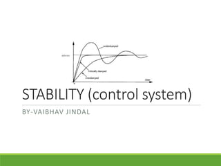
1. Stability of a system can be determined by observing its time response curve, with stable systems having oscillations that die out quickly or reach steady state fast. 2. Different types of stability include bounded input bounded output stability, asymptotic stability, absolute stability, and relative stability. 3. A system is stable if all poles are in the left half of the s-plane, marginally stable if poles are on the imaginary axis, and unstable if any poles are in the right half plane.

Recomendados
Recomendados
Mais conteúdo relacionado
Mais procurados
Mais procurados (20)
Semelhante a Stability of Control System
Semelhante a Stability of Control System (20)
Mais de vaibhav jindal
Mais de vaibhav jindal (17)
Último
Último (20)
Stability of Control System
- 1. STABILITY (control system) BY-VAIBHAV JINDAL
- 2. Physical Meaning of Stability
- 3. Introduction Stability of any system is a very important characteristic of any system . In Control System STABILITY cab be judged by observing the time response curve. (Which is basically depends on location of poles) Generally for a stable system oscillations must die out as early as possible or steady state should be reached fast. (in time response curve)
- 5. S-Plane and Time Response Curve 0<ζ<1 Under Damped System ζ =0 Undamped System ζ=1 Critical Damped ζ>1 Over Damped System
- 6. Stability Bounded Input, Bounded Output: Output must be bounded for bounded input. Asymptotic Stability: If system input is remove from the system, then output of system is reduced to zero. absolute Stability: A system is stable for all values of system parameters for bounded output. (Define in terms of location of poles) [Routh Hurwitz, Rout locus & Nyquist Plot] Relative Stability: This is a quantitative measure of how fast system oscillation die out with time and how fast steady state reached. (Define in term of Damping Ratio, Gain Margin and Phase Margin) System having poles away from the imaginary axis of S-Plane, in negative direction, has higher stability. [Bode Plot & Nyquist Plot]
- 7. Conclusion I 1. For a stable system, all roots of characteristic equation (Poles of the system) must lie in negative half of s plane. 2. If roots lie on imaginary axis, system is called marginally stable or limitedly stable. 3. If roots lie on the positive half side of s-plane, system if un-stable. 4. If there are repeated poles or roots on imaginary axis, then also system is un-stable. 5. If poles moves away from imaginary axis towards the left of s-plane the relative stability of system is improves. Im Re Stable Un-Stable
- 8. System T(s)= 𝐶(𝑠) 𝑅(𝑠) At least one of the system pole is in right half of s-plane At least some of the system poles are on the imaginary axis, the rest being in left half of s-plane All the system poles are inside the left half of the s-plane UNSTABLE ASYMPTOTICALLY STABLE At least one of the system poles on the imaginary axis is present in the form of a pole in R(s) SYSTEM EXHIBITS INSTABILITY DUE TO RESONANCE At least some of the system poles are repeated on the imaginary axis. UNSTABLE All poles on imaginary axis are simple and none of these poles are present in input R(s) NON-ASYMPTOTICALLY STABLE MARGINALLY STABLE
- 9. Routh Hurwitz Stability For a stable system all elements of first column in Routh table should have same sign(either “+” or “-”). “If Characteristics Equation contain only even power of S “ or “elements of any odd complete row of Routh table is zero” represents system will contain at least one pair of poles on imaginary axis (System has undamped natural frequency), system is marginally stable. Note: Routh is only applicable for closed loop system and for implementation of Routh table coefficient of characteristics equation. Should real
- 10. Bode Plot Gain Margin Phase Margin Stability ω 𝑔 < ω 𝑝 +ve dB +ve Stable ω 𝑔 = ω 𝑝 0 0 Marginally Stable ω 𝑔 > ω 𝑝 -ve dB -ve Un-Stable Gain Margin= -[20 log|G(jω 𝑝).H(jω 𝑝)|] Phase Margin=180+ ∠ G(jω 𝑔).H(jω 𝑔) ω 𝑔= Gain Cross over frequency ω 𝑝= Phase Cross over frequency Bode plot is draw on Semi-log graph for open and closed loop system both.
- 11. Nyquist Plot Relative Stability Gain = 1 |G(jω 𝑝).H(jω 𝑝)| Gain Margin(dB)= -[20 log|G(jω 𝑝).H(jω 𝑝)|] Phase Margin=180+ ∠ G(jω 𝑔).H(jω 𝑔) ω 𝑔= Gain Cross over frequency ω 𝑝= Phase Cross over frequency
- 12. Nyquist Plot Relation between Open and Close Loop System System Zeros Poles Open System G(s)H(s)= 𝑺+𝟏 𝑺+𝟓 -1 -5 Close Loop System (-ve Feedback) G(s)H(s) 1 + G(s)H(s) = 𝑆 + 1 2𝑆 + 6 -1 -3 Characteristics Equation 1 + G(s)H(s)= 2𝑆+6 𝑆+5 -3 -5
- 13. Nyquist Plot Absolute Stability 𝑁 𝑖𝑠 𝑒𝑛𝑐𝑖𝑟𝑐𝑙𝑒𝑚𝑒𝑛𝑡 𝑜𝑓 𝑝𝑜𝑖𝑛𝑡 (-1+j0). N=-1 [For clockwise N is –ve and anti-clockwise N is +ve]
- 14. Nyquist Plot 𝑁 = 𝑃+ − 𝑍+ Where, N=Total no. of encirclement of point (-1+j0). [For clockwise N is –ve and anti-clockwise N is +ve] 𝑃+=Positive poles of characteristic equation(Poles of open system) [Find from given transfer function]. 𝑍+=Positive zero of characteristics equation (Poles of closed loop system) [Find from above equation]
- 15. K=3, Stable K=7, Unstable
- 16. The Relative Stability of Feedback CS The verification of stability using the Routh-Hurwitz criterion provides only a partial answer to the question of stability----whether the system is absolutely stable. In practice, it is desired to determine the relative stability. - The relative stability of a system can be defined as the property that is measured by the relative real part of each root or pair of roots.
- 17. THANK’S MERCI
Notas do Editor
- Different ways of defining Stability BIBO: For any LTI system “ Any LTI system will be stable if and only if the absolute value of its impulse response g(t), integrate range will be finite. 0 ∞ 𝑔 𝑡 𝑑𝑡=𝐹𝑖𝑛𝑖𝑡𝑒 Relative stability: Degree of stability (i.e. how far from instability) • A stable linear system described by a T.F. is such that all its poles have negative real parts