1. Lewis Growth Model and China’s Industrialization
Kazuhiko Yokota
Nazrul Islam∗
Abstract
This paper examines China’s development experience in the light of Lewis’s growth
model. It first peruses Lewis’s own writings and those of Fei and Ranis in order to
identify the main predictions of the Lewis’s model. The paper next considers the
problems that arise in checking the validity of these predictions in general and in the
particular case of China. Finally the paper examines actual Chinese data. In particular it
examines whether Chinese wage data conform to the Lewis’s prediction regarding the
long-term shape of the wage curve. Overall the findings tend to support the predictions of
the Lewis model, though there remain many issues that need to be further investigated.
JEL Classification: O, P
Keywords: Lewis model; China; Development; Duality; Wage curve
October 11, 2005
∗
The authors are Associate Research Professor and Research Professor, respectively, at International
Centre for the Study of East Asian Development (ICSEAD), Kitakyushu, Japan. This is a very preliminary
version of the paper. Please do not quote. Send your comments to the authors at nislam@icsead.or.jp and
yokota@icsead.or.jp

2. 1. Introduction
This paper examines China’s development experience in the light of Lewis’s growth
model. It first peruses Lewis’s own writings and those of Fei and Ranis in order to
identify the main predictions of the Lewis’s model. It considers both the closed economy
and the open economy versions of the model. The perusal indicates that the main
prediction of the model remains the one derived from the basic closed economy version
that suggests that the modern sector wage curve should remain fairly flat for quite some
time before reaching a turning point and starting to rise. The wage curve for the
traditional sector meanwhile can witness an upward increase from an earlier point of time
even through remaining below the modern sector wage in terms of absolute level.
Testing these predictions however pose considerable challenges, as recognized by
Lewis himself and other researchers. These problems are even more serious with respect
to China because of it several specific institutional characteristics, such as the practice
and legacy of central planning, restrictions on urban-rural migration, changes in the
jurisdiction of urban and rural counties, establishment of modern industrial enterprises in
rural areas in the form of Township and Village Enterprises (TVE), etc. All these special
aspects of the Chinese situation add to the list of complications that arise in examining
reality through the prism of the Lewis model.
The paper examines a wide variety of Chinese data, focusing on the data on wages. It
offers graphical presentation of the relevant wage curves and provides accompanying
computational results based on Fei and Ranis’s decomposition of the growth rate of the
modern sector in terms of capital growth rate, direction of technological bias, and growth
rate of the total factor productivity. The paper begins by examining the national data
disaggregated by three broad sectors, namely primary, secondary, and tertiary. It next
moves to consider data from two different types of provinces, with one being a fast
growing coastal one (namely Shanghai) and the other being an slow growing inland
province (namely, Gansu). Overall the data tend to support the predictions of the Lewis
model. The modern sector wage curves do tend to be flat or very slow rising for a long
period of time before turning points are reached. In that sense Chinese development
1

3. experience does vindicate the validity of the Lewis model as a description of the reality.
However, many conceptual and data issues remain to be overcome before firmer
conclusions can be reached.
The discussion of this paper is organized as follows. Section 2 offers a brief
recapitulation of the salient features of Lewis model in order to set the background for the
discussion of this paper. Section 3 offers as perusal of Lewis’s own writings to determine
the predictions of his model. Section 4 extends the perusal to the writings of Fei and
Ranis, who have played the most active role in amplifying on and using the Lewis model.
Section 5 discusses the problems faced in confronting reality with Lewis’s model in
general and in particular with respect to China. Section 6 presents the empirical analysis
and the results. Section 7 concludes.
2. Lewis Model of Growth: A brief recapitulation
Exactly half a century ago, in May 1954, Arthur Lewis published his article,
“Development with Unlimited Supply of Labor” in the journal Manchester School. This
article and his subsequent writings gave rise to the famous “Lewis Growth/Development
Model,” the hallmark of which is the assumption of a dual structure of the economy.1
Various terminologies have been used to express this dualism. Among them are urban-
rural, capitalist-non capitalist, modern-traditional, agricultural-industrial, etc. Lewis
himself started with “capitalist-non capitalist” characterization of this duality, but later
recognized the possibility of other characterizations. As Lewis (1972) explains, the
difference between the two sectors is analytical, and not descriptive. The first analytical
difference between the two sectors lies in the fact (assumption) that same type of labor
has much higher (labor) productivity in one (say modern) sector than in the other (say
traditional) sector. Thus shift of labor from the traditional sector to the modern sector can
therefore augment the total output of the economy. The second analytical difference
between the two sectors lies in the fact (assumption) that the traditional sector is
characterized by the presence of ‘surplus labor,’ in the sense that withdrawal of this labor
does not lead to a reduction in the total output of the traditional sector. This has two
1
See Lewis (1954 and 1955) for original exposition of the model.
2

4. important implications. First, under this condition the entire output produced in the
modern sector by a unit of labor transferred from the traditional sector is an addition to
the economy aggregate output, and not just the difference between a laborer’s output in
the modern sector and the output lost in the traditional sector as a result of his or her
transfer from the latter to the former. Second, the opportunity cost of labor to be engaged
in the modern sector in terms of foregone output in the traditional sector remains constant
(and negligible), so that it does not have to offer higher wages to engage more labor. In
short, the modern sector faces an almost perfectly elastic supply of labor at the going
wage rate. The combination of the above assumptions imply that the economy will
witness a much larger surplus accumulated in the hands of the entrepreneurs of the
modern sector, and assuming that they invest at least a constant proportion of the surplus,
the economy will witness higher rate of investment and hence of growth.
Since the appearance of Lewis growth model based on the assumptions above, many
debates have been waged concerning the meaning and validity of these assumptions. The
recent symposium organized by the journal Manchester School to celebrate the 50 years
of Lewis 1954 article provides a good recent overview of where these debates stand and
what their impacts have been.2 In this paper however we are not concerned about these
debates. We want to accept the model as it is, and find out whether and how these can
help in understanding the Chinese experience of industrialization. In a sense, China
should have been the obvious case to check out the Lewis model of growth. Interestingly,
though some work in this connection has focused on Taiwan, not much research had been
done on China.3
3. Predictions of the Lewis model
There are different approaches to take. One would be to think of examining directly
the assumptions of the model. However, as Milton Friedman is famously contends, it
does not matter whether or not the assumptions are realistic. The important thing is
2
See in particular, Kirkpatrick and Barrientos (2004), Fields (2004), Figueroa (2004), Ranis (2004), and
Tignor (2004).
3
Among few papers that The only paper that we could find that related the Lewis model with China is by
Yingfeng Xu (1994) appearing in China Economic Review. This paper titled, “Trade Liberalization in
China: A CGE Model with Lewis Rural Surplus Labor.”
3

5. whether the predictions of the model prove to be correct. No matter whether or not we
agree with Friedman’s epistemological position, in confronting Chinese industrialization
experience with Lewis model, we can indeed focus on the predictions rather than on the
assumptions directly. This brings us to the questions of the predictions of the Lewis
model.
Lewis (1972) explains more explicitly that there are three different variants of the
model. In Model One the economy is closed and there is no trade between the two sectors.
In this model the first turning point is reached when “the labor supply ceases to be
infinitely elastic and the wage starts rising through pressure from the non-capitalist
sector.” (p. 83) He also identifies a second turning point, which is reached when “the
marginal product is the same in the capitalist and non-capitalist sectors, so that we have
reached the neo-classical one-sector economy.” (p. 83)4
Model Two continues with the closed economy scenario, but now assumes that the
two sectors produce different goods and hence trade with each other.5 This brings into the
analysis the additional issue of terms of trade between the two sectors, and it now creates
the possibility that growth in the modern sector can get choked because of adverse shift
in the terms of trade even when the pool of surplus labor has not been exhausted.6 This
will happen particularly if the productivity growth in the agricultural sector lags much
behind that in the industry sector.7 However, even if the terms of trade rise (deteriorates)
4
In a footnote, Lewis notes that “The second turning point is exactly the same as in Fei and Ranis (1964, p.
201-5). The definition of the first turning point is also the same, but the mechanism for reaching it is
different, since Fei and Ranis are working with Model-II, in which the capitalist sector depends on the non-
capitalist sector for agricultural products.” (Lewis 1972, p. 83)
5
In explaining the set up, Lewis further notes that “Thus our specifications are altered. The division
between the two sectors now turns on commodities rather than on capitalists; it makes no difference to us
whether there are capitalists in the slow-growing sector, provided we specify that their profits are not
reinvested in the fast-growing sector. What we still need is a substantial initial difference between real
wages in the two sectors, so that labor is not initially a problem to the fast-growing sector. Following the
conventions, we will now divide the economy into an industrial and an agricultural sector, with industry
paying significantly higher wages than agriculture.” (Lewis 1972, p. 92)
6
As Lewis explains, “In this version our two sectors produce different commodities and therefore trade
with each other. Thus the capitalist sector faces the additional hazard that it may be checked by adverse
terms of trade, arising out of the pressure of its own demands, long before any shortage of labor begins to
be felt.” (Lewis 1972, p. 91) He further notes that “This is the version, which has been worked out in great
detail by Fei and Ranis working with models in which each of the variables is or can be precisely
determined. Jorgenson and others also prefer to work with this model.” (p. 91)
7
Following Johnson’s trade model, Lewis shows that the terms of trade between the two sectors will
remain constant if the relative growth rates of industry and agriculture are the same as the relative income
elasticities of demand for product of these two sectors. (p. 93)
4

6. for the industry, its expansion may not cease if the productivity growth in this sector
outpaces the rate of deterioration in the terms of trade.8 The concrete outcome will then
depend on the concrete paces of productivity increase in the two sectors and the resulting
concrete impact on the terms of trade and movement of the real wage.9
Model Three allows international trade (an open economy situation) so that a rapidly
growing industrial sector faced by a too slow agricultural sector can import agricultural
products and pay for the imports by exporting its own product. However, Lewis notes
that in order to export more, the producers may have to lower the prices thus causing a
dent in the profit margin. Thus the prospects and propensity of export becomes a crucial
determinant in this scenario.10 He surmises that “a country must plan its development in
such a way as to be sure that its exports will keep pace with needed imports. If it fails to
do this, the rate of growth of output will be constrained by the rate of growth of export
earnings.” (p. 94) The above shows that Model Two and Model Three basically add some
qualifications to the basic predictions arising from Model One.
In this discussion of the open economy scenario, Lewis (1972) focuses on the terms of
trade issue. However in the original paper’s discussion of the open economy scenario,
Lewis (1954) focuses on possible factor movements. Thus Lewis notes that reaching of
the turning point and rise of the wage may be checked by mass immigration and export of
capital.11 The checking influence of export of capital can be offset “if the capital export
cheapens the things which workers import, or raises the wage costs in competing
countries. But it is aggravated if the capital export raises the cost of imports or reduces
costs in competing countries. So Lewis points to a connection between factor flows and
8
As Lewis (1972, p. 93) explains, “even if the terms of trade are rising, industrial expansion will not
necessarily cease. Productivity is rising in the industrial sector, so if real wages (w/c) are constant, the
profit margin will not fall unless the terms of trade rise faster than industrial productivity.”
9
As Lewis (1972, p. 93) explains, “Real wages cannot be constant if agricultural productivity is rising
significantly, since this would be moving the factoral terms of trade against industry. So what will happen
to profits in any particular case will depend on a race between agricultural productivity, industrial
productivity, real wages (which may rise on their own for exogenous reasons), and the commodity terms of
trade. If one makes precise assumptions about these magnitudes one can get precise answers, as Fei and
Ranis have done.”
10
The following is how Lewis (1972, p. 94) argues: “However, in order to export more it may have to
lower its prices, thus squeezing its profits. Its real wages, in terms of agricultural products, are fixed by
definition. If we take as given the propensity to import and the inflexibility of the agricultural sector, we
can see that the possible rate of growth of such an economy is determined by its propensity to export.”
11
As Lewis (1954, p. 190) puts it, “The country is still surrounded by other countries which have surplus
labor. Accordingly, as soon as its wages begin to rise, mass immigration and the export of capital operate to
check the rise.”
5

7. terms of trade that a country faces. Lewis (1954) noted the possibility of import of capital
too. He notes that capital inflow will not generally raise wages as long as surplus labor
exists. (p. 191)12
4. Extension of Lewis model’s predictions by Fei and Ranis
Fie and Ranis (henceforth FR) have played an important role in expanding and
extending the Lewis model. As noted above, they impose a “product dualism” on the
original Lewis dualistic model in order to introduce in the model the issue of terms of
trade. It also makes the model more amenable to the influence of international trade
opportunities. According to the “product dualism” the products produced by the two
sectors are different. Extending Lewis’ idea, FR identifies or proposes four turning points.
These are: (a) commercialization point, (b) reversal point, (c) export substitution point,
and (d) switching point. (p. 290)
The Commercialization point is basically the same as the first Turning Point
mentioned by Lewis above, though FR amplifies on further properties of this point in the
context of an open dualistic model.13 The “reversal point,” according to FR, is the pointy
at which the traditional sector (which FR equates with agricultural sector) starts to
12
“The importation of foreign capital does not raise real wages in countries which have surplus labor,
unless the capital results in increased productivity in the commodities which they produce for their own
consumption.” (Lewis 1954, p. 191)
13
RF explain that commercialization “indicates the end of the surplus labor condition. From this point on,
the real wage in agriculture equals the marginal product of labor, which signifies that labor is now a scarce
factor and the wage increases rapidly.” (p. 290) RF further explain that the definition of this point remain
unchanged for the open economy. As they put it, “this concept (of commercialization point – ni) is also
applicable to the open dualistic economy.” (p. 290) However they add that “in the open economy case, the
arrival of the commercialization point is found in combination with the ‘push’ effects of technological
change in agriculture and the ‘pull’ of industrial labor demand, both augmented by the access to the
international economy.” (p. 290) They further note that “the open economy commercialization point at
which the MPL exceeds the IRW at Wa arrives earlier the faster the upward shift of the MPL , the slower
the rate of population growth, the slower the upward creep in the institutional real wage, and the faster the
demand for labor increases in the industrial sector.” (p. 290) According to them, “the open economy
commercialization point is the end of the natural austerity typical of the unlimited supply of labor condition.
After the commercialization point the savings rate and the GDP growth rate level off. Furthermore, in an
open dualistic labor surplus economy the commercialization point is also likely to change the structure of
international trade. The external orientation of the industrial sector – previously based on entrepreneurs
taking advantage of cheap labor – gives way to the incorporation of skills and capital goods as the basis of
exports. Simultaneously the orientation of the industrial sector shifts to satisfy the growing domestic market
for industrial consumer goods.” (p. 290)
6

8. witness absolute decline in its labor force.14 The next point according to RF is the “export
substitution point.” According to their set up, industrialization of the dualistic economy
begins with import substitution, and after a while the country progresses to the “export
substitution” stage.15 Finally there is the “switching point,” when, according to RF, the
country becomes a net importer of agricultural goods.16
14
“The second turning point is the reversal point signifying an absolute decline in the agricultural labor
force.” (p. 292) “The analysis of chapters 3 and 7 … shows that when the growth of the industrial labor
force (ηW ) is sustained long enough at a level above the growth rate of the total labor force (η P ), not only
does θ = W/P increase continuously, but a reversal point is reached when the absolute increase of the
agricultural labor force gives way to an absolute decline.” (pp. 292-293) They further explain that “when
the supply of land is fixed, the arrival of the reversal point signifies that the law of diminishing returns is
beginning to work in the reverse direction, as the marginal and average productivities of labor in both
sectors increase even when technological change is stagnant. This implies that pressure exists to adopt
labor-saving technology in agriculture since there is a ‘shortage’ of manpower under the original
technology” (p. 293)
15
“The third turning point in an international context is the export substitution point… During the long
period of growth prior to transition growth, the economy is land based and fueled by primary product
exports. During the import substitution phase which characterizes the initial period of transition growth, the
open economy relies on agricultural land-based exports to build up and sustain its import substitution
industries. The import substitution strategy usually adopted by the government (high tariff protection for
domestic market by the official exchange rate, artificially low domestic interest rate, etc.) encourages the
use of foreign earned by traditional exports to develop and subsidize import substitution industries. Export
substitution occurs when labor intensive manufacturing replaces traditional exports as the dominant export
items of the economy.” (p. 294)
“When the domestic markets for industrial consumer goods are supplied almost exclusively by import
substituting industries, the import substitution phase comes to an end. In the case of a small labor surplus
economy, the natural development is the emergence of an export substitution phase – selling labor-
intensive manufacturing exports to the world market. This transition is facilitated by changes in
government policy to promote (for example realistic exchange rates) base on labor efficiency.” (pp. 294-
295)
“The emergence of the export substitution phase replacing the import substitution phase is a highly
important phenomenon for the labor surplus economy analyzed here. While the import substitution phase
was not conducive to full employment – leading to the ‘necessary’ conflict between employment and
growth – there is no such conflict when the export substitution phase arrives since labor is embodied in
exports, which is conducive to both rapid growth and full employment. As this process advances, it leads to
the ‘commercialization’ and ‘switching’ points, signifying the termination of the labor surplus condition in
the economy as a whole, as well as in the agricultural sector in particular.” (p. 295)
16
The final transition point in the transition of the open dualistic economy is the switching point. It is based
on the notion that countries at some time become net importers of agricultural goods. In general, the
phenomenon of land-based exports at the beginning of the transition to the modern industrial economy is a
temporary phenomenon. A ‘switch’ from an agricultural exporting to an agricultural importing economy is
bound to occur at some stage of the successful development process. But when it occurs, and on the basis
of what kind of agricultural performance, remains an all important issue. It matters greatly whether or not
existing reserves of agricultural productivity have been harnessed en route to successful balanced transition
growth in the LDC. The alternative is a failure of the total development effort – true for many
contemporary LDCs – or an unacceptable reliance on foreign capital.” (pp. 296-7)
“The array of government policy measures (for example, tariffs, exchange controls, etc.) adopted to
facilitate the import substitution process via the exclusion of foreign competition and the augmentation of
profits to the domestic industrialists are subject to change. Stabilization plus dismantling direct controls on
trade and exchange rates creates a more market oriented economy conducive to the utilization of the
7

9. Many of these additional turning points, particular the latter two, appear to be
particularistic, depending on the further assumptions that RF makes onto the basic Lewis
dualistic model, and hence may not be considered to be that general. (Further scrutiny is
necessary in order to clarify this point.) However this discussion already shows that it is
possible to draw more conclusions/predictions from the Lewis model once openness is
incorporated more fully into the model. This may however require assumptions that may
go beyond what the original model calls for.
As noted earlier, trade in goods and services is however not the only type of flows that
openness introduces to a closed economy. Other important flows are of capital,
technology, and even labor. FR provides a perceptive discussion of how these other flow
can affect the development process of a dualistic economy. (pp. 306-319) They think that
availability of foreign capital can have both quantitative as well as qualitative effects. The
quantitative effect refers mainly to the increase in the amount of capital that becomes
available to the developing dualistic economy, and this may quicken the process of
capital accumulation, absorption of the surplus labor, and thereby shortening the time
required for the economy to reach the Turning Point. Their discussion of the qualitative
effect of capital inflow is not as clear. It refers to the possibility that opens up for the
country to import capital intensive capital goods and thus to be free to engage its own
capital to produce labor intensive goods. However, this aspect referring to the physical
attribute of goods seems rather belong to the issue of trade and not capital inflow per se.
In this regard FR also point out that the beneficial impact of capital inflow may get
obviated by wrong policies pursued by the receiving country, as exemplified by India
which followed a capital-intensive industrialization policy and thus failed to make use of
its labor abundance. However, this point again was equally valid for the closed economy
model, and thereby does not represent an analytical novelty arising from the openness to
foreign capital inflow. FR recognizes the point.
economy’s abundant resource – surplus labor – via embodiment in labor-intensive industrial exports.
Concurrent to this, the open dualistic labor surplus economy is likely to move from the successful
exploitation of its agricultural potential to a long-term position as an agricultural importer as the industrial
sector becomes successful. The arrival of such a switching point signifies that the LDC ultimately
accelerates its industrial exports to acquire needed food and raw materials. Finally, an absolute decline in
the agricultural population shifts the policy focus towards labor-saving techniques in agriculture to prolong
the labor-using phase in industry as the economy gets ready for the skill- and capital-intensive phase.” (p.
296)
8

10. With regard to labor mobility, RF rightly notes that it is of lesser importance given the
restrictions on both the demand and supply sides. The impact on the dualistic economy
again depends on the policies pursued by the economy itself. They present the Philippines
as the “unsuccessful” case, which failed to make use of its surplus labor and let its skilled
labor to migrate. On the other hand, RF portrays East Asia as the “successful” case that
made good use of it surplus labor. They also mention of a “Returning Point” with regard
to migration as exemplified in particular by the experience of Taiwan, whose migrants
are now returning to the country. These empirical points are interesting. However, the
import of labor mobility for the model itself remains ambiguous. In general it is clear that
labor mobility to the extent that it allows the dualistic economy’s surplus labor to migrate
may bring the Turning Point nearer. On the other hand, if labor mobility rather makes it
easier for only the skilled labor to migrate, then such mobility may rather make transition
of the dual economy more difficult. The outcome therefore is not clear.
Finally RF comes to the issue of technology. They use their following basic equation
to discuss the issue:
(1) η P < ηW = η K + ( J + BL ) / ε LL
where, η P , η W , and η K are growth rates of population, workers in the modern sector,
and capital, respectively, J is the innovation intensity, BL is the factor bias (toward labor)
of production, and ε LL is the elasticity of the marginal productivity of labor. The
presence of BL suggests that the more labor biased technology the better for the dualistic
economy. RF explains that in the context of dualistic developing countries “J corresponds
to the adaptation of foreign technology to domestic production processes, which allows
output to increase without necessitating a rise in the domestic capital or labor stock.” (p.
313) On the whole, FR seems to advocate “appropriate technology.” They explain that
“appropriate is not necessarily small-scale or large-scale, labor-intensive or capital-
intensive, but that which fits the existing resource endowment at a particular point in time,
both with respect to technique choice and product quality.” (p.314)
9

11. Be that as it may, the implication of the technological possibilities arising from
openness remains again ambiguous. Much depends on the policies that the economy
pursues. In this regard they emphasize the necessity of removal of price distortions. They
portray East as the successful case in removing price distortions that allowed these
countries to make the best use of the technological opportunities. The also note the
remarkable capacity that Japan displayed in technological adaptation. This all may be
true, though the discussion smacks of post-fact theorization.
Overall therefore we see that incorporation of possibilities that emerge with opening
up does not change the story of the dualistic economy that much. In fact FR had informed
of this at the outset of their Chapter 8 announcing that “domestic balanced growth
remains the centerpiece of success in the open economy, even in relatively small country
cases.” (p. 283) However, we also see that “the open economy can (indeed) be of
considerable help loosening the strait-jacket of resource constraints and inherited autarky,
aiding the domestically-driven growth of the dualistic LDC.” (p. 283)
How far this marginalization of the role of openness is valid can be an interesting
theoretical issue to examine. However, this paper is meant to examine the Chinese
growth experience in the light of the Lewis growth model. In doing so, we need to
consider open economy issues, both because Lewis himself and Fei and Ranis in
particular made interesting efforts to extend the model to an open economy situation and
because the Chinese recent growth itself has been achieved in an, by and large, open
economy situation. To the extent that such an analysis can also provide a check on the
validity of marginalization of openness, as suggested by FR above, will be a bonus.
5. Problems in empirical testing of Lewis model’s predictions
5.1 Problems in general
Thus the most important prediction of the Lewis model concerns the wage curve for
the modern sector. The model implies that the wage curve of the modern sector will
remain essentially flat or rising very slowy for a long time until the surplus labor of the
traditional sector has been absorbed in the modern sector. The point at which the surplus
labor gets exhausted and the modern sector wage curve starts to move up (from being
10

12. flat) is called the “Turning Point.” How long is this “long time” and how flat this
“essentially flat” curve has to be are questions of dispute of a secondary order. Earlier,
based on wage data of England, Japan, and Taiwan, Ranis showed that the experiences of
these countries conform to the Lewis model prediction. The modern sector wage curve
for these countries indeed remained more or less flat for about forty years, before the
Turning Point was reached.
However there are many problems with regard to testing the validity of Lewis model’s
prediction. One of these concerns determining the empirical counterparts of the
theoretical concept of dual sectors. As noted in Section 1, Lewis himself and the literature
have employed many different versions of this duality concept. Capitalist/non-capitalist,
modern/traditional, industrial/agricultural, etc, are just a few examples. No matter which
of these versions is preferred there is never a perfect match between them and the
empirical counterparts that are or can be employed given the availability of data.
Another issue concerns the definition of real wage itself. As Lewis (1972, p. 85)
himself noted, “Real wage has many meanings.” He drew distinctions among “cost of
living wage,” defined as (w/c), where w is the nominal (money) wage and c is the cost of
living; “factoral wage,” defined as (w/a), where a is “the income of the noncapitalist
worker;” “ratio of wages to prices,” defined as (w/p), where p is the index of the “price
received by capitalists;” product wage, defined (wL/vQ), where is the quantity of labor, Q
is real output, and v is the value added price of output; and finally (wL/pQ) which is what
product wages reduces to when no imported raw materials are used in production. (Lewis
1972, pp. 85-86) Coupled with all the different ways in which the sectors can be defined,
this shows the bewildering variety of combinations that can be adopted for empirical
testing the predictions of Lewis model.
5.2 Particular Problems with China
When it comes to China, there are additional problems arising from her various
institutional specifics. First of all, as explained earlier, the analytical modern-traditional
dichotomy is not the same as the empirical urban-rural dichotomy. This is more so in the
China. First of all, not all of urban sector is comprised of enterprises embodying modern,
11

13. industrial technology having higher labor productivity. A considerable part of the urban
sector is comprised of informal enterprises using primitive technologies. Similarly, not all
of rural sector, as administratively defined, is comprised of economic (agricultural or
otherwise) activities based on traditional, pre-industrial technologies. This is more so in
case of China, which has witnessed a phenomenal growth of Township-Village
enterprises (TVE) right inside what are administratively classified as rural areas. Yet
many of these TVEs employ industrial technology. Second, even the administrative
demarcations of urban and rural parts of the country have not stayed the same over time.
What was rural a few years earlier became urban due to administrative decisions
regarding the jurisdiction of cities and counties.
A (third) problem that is not of correspondence between analytical concepts and
empirical concepts, but of a significant departure from the analytical description of the
Lewis economy is as follows. The Lewis model assumes on an unrestricted flow of labor
from the traditional to the modern sector in response to the economic incentives. The
model does not allow for administrative or political restrictions on such flows. This
assumption does not hold true for China. For a long time China practiced what is called
the Registration System, under which people were not free to move from one location to
another. In particular rural people were not free to move to urban areas and take up
residence there. Over time many of these restrictions have been either removed formally
or enforced not so strictly, making it easier for rural residents to move to urban areas.
However, many such restrictions remains, and the situation still remains far removed
from the one postulated in Lewis model.
Finally there is the problem of the practice and legacy of central planning in China. As
we noted earlier, the initial idea of Lewis model was to explain the growth and expansion
of capitalism (or industrialization under capitalism) in developing countries. That might
have been one reason why researchers have not been that enthusiastic in examining
mainland Chinese growth experience from the viewpoint of Lewis model, even though
the model has been extensively used to study the growth process in Taiwan and also to
some extent of Japan. Since under central planning wages (as other prices) are
determined through fiat/command/administrative methods, it might have been thought
12

14. that Lewis model, which in a sense rely on market rationale, was not the appropriate
reference model.
However, as Lewis himself noted, industrialization in a dual economy faces the same
economic fundamentals even when it is carried out under alternative (non-capitalist)
institutions. In fact he mentions that was the experience of the (former) USSR (along
with that of the UK) which served as the empirical reference for him in his formation of
the model.17 Clearly, therefore Lewis thought his model to be applicable for analysis of
industrialization in a dual economy under socialism (central planning) too. However, in
considering the latter process, one has to keep in mind that the planners may not always
go by the economic fundamentals, and instead try to impose choices inspired by non-
economic, political or ideological considerations.
China’s situation is further complicated by the fact that it is neither under central
planning nor under entirely market conditions. Instead it is in a transition from the former
to the latter. On the one hand it makes the analysis, in particular interpretation of the
results more challenging. On the other hand, it offers more opportunities to find whether
and how institutional changes impact on the underlying economic processes of
industrialization.
6. Empirical Analysis and Results
We begin the analysis by examining the data at the aggregate level. Table 1 shows the
real GDP distinguished by three sectors, namely Primary, Secondary, and Tertiary.
According to the classification adopted by the Chinese statistical authorities, the Primary
sector comprises of agriculture and mining, Secondary of manufacturing, and Tertiary of
services. The Secondary sector can by and large be thought to be the “modern” sector of
the economy, employing industrial technologies. On the other hand, the Primary sector
can by and large be thought to represent the “traditional sector,” though mining, that is
included in this sector, may actually employ industrial technologies. Even agriculture in
China is becoming more machine based, as we will see later. Relatively more
17
As Lewis (1972, p. 87) puts it: “When the first article was written, the historical wage data uppermost in
my mind were those for the cost of living wage in Great Britain in the first half of the nineteenth century,
and the USSR in the 1930s.”
13

15. problematic is the Tertiary sector, which may include enterprises based on either
industrial technology or pre-industrial traditional technologies. It is therefore difficult to
place the Tertiary sector in terms of the modern/traditional or industrial/pre-industrial
divide.
The graph in Figure 1 shows the dramatic increase in the volume and its share in GDP
of the Secondary sector. This reflects the process of industrialization that China is
undergoing. The graphs show that there has been a clear acceleration in this regard
beginning 1991. The volume of the Tertiary sector’s output has also been increased,
though nowhere at a rate similar to that of the Secondary. The Primary sector’s output has
increased at an even slower pace.
Figure 2 shows the employment pattern. It shows that in terms of employment, the
Primary sector still surpasses the Secondary sector in importance. The total volume of
employment in the Primary sector has remained relatively stable over the long period of
time considered (1978-2003). The graph also shows that employment in the Secondary
sector has increased but not so dramatically as its output. By contrast, employment in the
Tertiary sector has experienced steady increase and since 1994 surpassed the Secondary
sector in terms of total employment.
Figure 3 shows what is already suggested by Figures 1 and 2. We see a dramatic rise
in labor productivity in the Secondary sector, particularly beginning 1991. The labor
productivity in the Secondary sector fat surpasses that in the Tertiary and Primary sectors,
and it undergoes a surge beginning 1991. By contrast labor productivity in the remaining
sectors experience only very sluggish growth.
Figure 4 shows the wages in the three sectors and for the economy as a whole. We
notice that unlike labor productivity, real wages in all the sectors seem to display
somewhat similar pattern. Wages in all the sectors experience faster increase beginning
1993. In terms of level and growth, wages in the Secondary and Tertiary sectors seem to
move very closely. However, surprisingly, in view of the labor productivity information
provided by Figure 3, wages in the Tertiary sector, accordingly to these data, exceed
those in the Secondary sector and certainly those in the Primary sector.
Broadly, these wage curves do display the pattern suggested by the Lewis model.
After rising at a sow pace for a long time, they start rising at a much faster rate after
14

16. reaching what according to Lewis model would be the First Turning Point. However, the
graphs also show that the Chinese economy is nowhere near reaching the Second Turning
Point, where the marginal product of the modern sector equals that of the traditional
sector and is reflected in the approximate equality of the wages in the modern and
traditional sectors. Figure 4 shows that the gap between wages of the Secondary and
Tertiary sector on the one hand and of the Primary sector on the other is actually rising.
According to Lewis model, the (first) turning point will be reached provided growth
rate of employment in the modern sector exceeds the growth of the total labor force.
Denote Primary, Secondary, and Tertiary sectors by the numerals 1, 2, and 3. Then,
assuming that the Secondary sector represents the modern sector, the above suggests that
employment growth rate in the Secondary sector (η 2 ) has to exceed the total labor force
growth rate ( η1+ 2+ 3 ).
Table 1 shows these and other relevant growth rates for different sub-periods. The first
sub-period of 1978-83 represents the initial reform period, when reforms were focused
mainly on the rural sector. The next sub-period of 1984-1988 represents the beginning
years of the industrial reform. The third sub-period of 1989-1991 represents the years of
political turmoil preceding and following the Teinamon incident. The fourth sub-period
of 1992-2001 represent years of continued industrial reform leading to China’s accession
to WTO. The final sub-period, still very short, represents post-WTO years. We see that
except for the abnormal sub-period of 1989-91, η 2 did indeed exceed η1+ 2+ 3 in all the
sub-periods.
As noted earlier, Fei and Ranis provides a decomposition of the employment growth
rate in terms of growth rate of capital (η K ), labor-bias of technical change (B), and TFP
growth (J). This decomposition allows seeing more clearly the source of employment
growth or the lack thereof. It thus helps thinking of policy interventions. Table 2 presents
such decomposition of η 2 for all the sub-periods. We see that most of the employment
growth was due to capital accumulation. The negative values of B show that technical
change bias was against labor rather than favoring labor. Finally, the values of J show
that total factor productivity growth was generally positive, except during the first sub-
period.
15

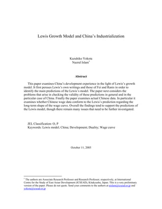
17. We noticed earlier the difficulty with placing the Tertiary sector in the
modern/traditional divide of the economy. Assuming that it is part of the modern sector,
it should also witness a faster employment growth in order to help reach the turning point.
Table 1 indeed shows that employment growth rate of the Tertiary sector (η 3 ) was
indeed higher than the employment growth for the overall economy (η1+ 2+ 3 ) for all the
sub-periods. Table 3 offers a decomposition of η 3 using Fei and Ranis formula. We
again see that capital accumulation has been the main source for the employment growth.
Technological bias even in this sector has been against labor, as manifested in the
negative values of B. Finally, we notice that total productivity growth had a relatively
less important role in this regard in the Tertiary sector than in the Secondary sector.
One important characteristic of recent development of the Chinese economy has been
unevenness of the growth and industrialization process across different provinces
resulting in enormous regional disparity. This can be seen clearly from the information
presented in Table 4. We see that the per capita income ranged from as high as 46,718
yuan in Shanghai province to a low figure of only 3603 yuan in Guizhou province. In
other words the per capita income of the richest province was about 13 times higher than
that in the poorest province. This is an enormous disparity to be observed inside the same
country anywhere is the world. Also, the difference is not only in terms of income. The
coastal and the interior provinces of China seem to be experiencing entirely different
development processes. While the former has become very an integrated part of the
global economy, the latter still remains isolated and looking inward. It is therefore
necessary to go beyond the aggregate level and see how different the processes in
different provinces appear when looked from the viewpoint of the Lewis growth model.
In order to do so we choose two provinces from two extremes of the income
distribution. One is the province of Shanghai, the richest province, and the other is Gansu,
the next to the poorest province.18 One is a coastal province, while the other is an interior
province. (The map in Figure 5 shows the geographical location of these and other
provinces of China.)
18
We could not select Guizhou province for this purpose, despite our original intention to do so, because of
data paucity for that province.
16

18. Figure 6 presents the manufacturing wage information for two rich provinces, namely
Shanghai and Beijing, and two poor provinces, namely Guizhou and Gansu. We see that
wage curves for Shanghai and Beijing undergo a sharp upturn beginning 1997. Wage
curves for Guizhou and Gansu also undergo an up turn beginning that year, but nowhere
as sharp as is the case with the richest provinces. It may be noted that all these provinces
had very similar wages at the beginning of the period (i.e., in 1985). In fact it is of much
interest to note that wages in Gansu were higher than in both Shanghai and Beijing. So
the dramatic divergence in average wages in entirely a recent phenomenon.
Figure 7 shows per capita income for Shanghai and Gansu provinces. We see the
dramatic increase in the per capital income in Shanghai, particularly beginning 1991,
while the per capita income of Gansu does not experience any such spurt. Figure 8 shows
the agricultural and non-agricultural population in Shanghai. We see that an absolute
decline in the size of the agricultural population and a steady increase in the size of the
non-agricultural population. Figure 9 shows the size of urban and rural population in
Gansu province. We see that Gansu also witnesses considerable increase in the size of its
urban population. It witnesses a decline in the size of the rural population too, though not
by that much.
Table 5 presents employment growth rates for various sectors of the Shanghai
province. We see from Table 5 that the Tertiary sector employment growth rate (η 3 )
always exceeded the total employment growth rate (η1+ 2+ 3 ). This however cannot be said
with regard to the Secondary sector employment growth rate ( η 2 ), which, as Table 5
shows, proved to be smaller than η1+ 2+ 3 in all the three recent sub-periods. This shows
that Shanghai has reached the stage where the service sector supplants the manufacturing
sector as the main driving force of the economy.
Tables 6 and 7 provide the Fei and Ranis decomposition of the Secondary and Tertiary
sector employment growth rates, respectively, of the Shanghai province. We see that in
each case, capital accumulation is the main force driving employment growth.
Technological bias seems to be against labor, particularly in the Secondary sector in the
more recent periods, accompanied by high total factor productivity growth. The Tertiary
17

19. sector in contrast has used more labor-favoring technology, suffering at the same time
from lack of TFP growth.
Tables 8, 9, and 10 provide analogous results for Gansu province. Table 8 shows both
η 2 and η 3 to exceed η1+ 2+3 in all the sub-periods, except the turmoil period of 1989-1991.
Table 9 provides the Fei-Ranis decomposition of η 2 . Data are patchy for Gansu, making
it not possible to conduct this decomposition for all the sub-periods, particularly the
beginning ones. Broadly, we see again capital accumulation to be main force driving
employment growth. The technology bias appears to be consistently against labor. There
does not seem much role for TFP growth in case of the Tertiary sector, though in the
Secondary sector witnesses some positive development in this regard in the more recent
sub-periods.
We noted in Sections 3 and 4 that openness, making international trade and factor
flows possible, creates many possibilities for modification of the basic predictions of the
Lewis model. The comparison between Shanghai and Gansu can be helpful in seeing the
impact of openness, because these two provinces also present different degrees of
openness and integration with the outside world.
Figure 10 shows the export and import figures for Shanghai. We see the explosive
growth of both exports and imports beginning particularly 1993. Also imports begin to
exceed export in Shanghai from 1999 onwards. Figure 11 presents similar information for
Gansu province. We see growth in export and import for Gansu too, however not as
dramatic as for Shanghai. Only in very recent years that it seems that exports and imports
are gaining momentum in Gansu. However, the absolute magnitudes are still very paltry,
so that small changes can get easily magnified, and discerning robust trends may be
difficult. Unlike in Shanghai, imports always exceed export in Gansu.
Figure 12 provides the decomposition of import in Shanghai in terms of agricultural
and capital goods. It shows clearly that most of the import is of capital goods. By contrast
import of agricultural goods remains almost unchanged. Figure 13 provides analogous
decomposition for the Gansu province. Again we see most of the import to be of capital
goods. However the absolute magnitudes are very small. Import of agricultural goods by
Gansu province has remained either unchanged or even declined.
18

20. In order to see the role of imported capital in the growth process, we expand the
production function to allow two types of capital, domestic and imported. Let K Di , K Mi ,
represent domestic capital and imported capital, respectively. The production function (in
Cobb-Douglas form) can then be written as:
(2) (
Y = A K D− β K M
1 β
)
α
L1−α .
Noticing the elasticity of marginal product of labor this case is ε i = 1 − (1 − α )γ , we have
the following equation providing decomposition of the output growth rate into its various
sources:
(3) ˆ ˆ ˆ ˆ ˆ
Y = A + α (1 − β ) K D + αβ K M + (1 − α ) L .
Table 11 and 12 provide decomposition of growth in Shanghai and Gansu,
respectively, following equation (3). From Table 11, we see that TFP growth plays a very
important role in the growth of Shanghai. It also shows significant contribution from
imported capital. In fact, positive contribution of imported capital contrasts with the
negative contribution of domestic capital. This shows that composition of capital in
Shanghai is changing towards imported capital.
Table 12 shows that the situation in these regards is very different in Gansu. First of
all the role of TFP growth is very limited. Second most of the contribution is from
domestic capital, with a minuscule role for imported capital. This suggests an association
between higher TFP and use of imported capital.
It is also interesting to note that contribution from proves to be negative in both the
provinces during most of the period, except the very recent year. This is borne out by
actual labor force data, as presented in the Appendix Table.
7. Conclusions
This paper examined the Chinese development experience from the viewpoint of
Lewis growth model. It first identified the main predictions of the model and then
confronted the Chinese data to check the validity of these predictions. The fundamental
19

21. prediction of the Lewis model is that the wage of the modern sector will rise only very
slowly at the beginning until when a turning point is reached signifying exhaustion of the
‘surplus’ labor contained in the traditional sector. Introduction of internal trade and
external trade and factor flows offer only different modifications to this basic prediction.
The empirical investigation of the paper begins with Chinese data at the national level,
disaggregated in terms of Primary, Secondary, and Tertiary sector. The wage curve for all
these sectors are found to display the distinct Lewis pattern, rising only slowly for a long
period before a Turning Point beyond which the curves rise steeply. The turning point is
more pronounced for the Secondary and Tertiary sectors than for the Primary sector,
which is what is expected.
This pattern seems to hold both for the rich coastal provinces, as exemplified by the
data of Shanghai, as well as for poor interior provinces, as exemplified by the data of
Gansu. However, the turning point is much sharper for Shanghai than for Gansu. This
suggests that import of agricultural product as a mitigating force (with respect to rise in
wages) did not play much of a role. China herself being a large agricultural country
having comparative advantage in production of many pertinent agricultural goods may
have played a role in this regard. Instead, faster capital accumulation, both domestic and
of foreign source, have led to sustained increase in non-agricultural employment. Higher
TFP growth, in part due to the use of imported capital, has made it possible to sustain
growth while paying out higher wages.
The turning point for the interior province of Gansu proves less sharp because of
smaller sizes of the Secondary and Tertiary sectors relative to the Primary sector. The
fact that the wage curve experiences an upward turn even when the rural sector remains
large is by itself an interesting finding. It remains of much interest to see how the wage
curves behave in the coming years in the interior provinces.
Overall therefore the data lend support to Lewis’s basic proposition that the
economies of populous developing countries, such as of China, are characterized by a
duality, instead of being characterized by perfect mobility and equalization of factor
returns across sectors as assumed by the neoclassical growth model. It is this duality that
allows the modern sector to expand for a significant period of time without having to feel
pressure of rising real wage rates.
20

22. Of course there remain many conceptual and data issues that remain to be sorted out
before these conclusions can be made firmer. We hope that future research will indeed
help us to do so.
21

23. Technical Appendix
Appendix 1: Derivation of Fei-Ranis Condition
Ranis and Fei (1997) identify the conditions for industrialization in which the
minimum labor reallocation condition for successful development becomes
η P > ηW ( Failure)
η P = ηW ( Stagnation)
η P < µW ( Industrialization)
BL + J
η P < ηW = η K +
ε LL
where ηP is the growth rate of total population, ηW is the growth rate of labor forth in urban
sector, ηK is the growth rate of capital stock (capital accumulation) in urban sector, BL is the
labor-using bias of innovation, J is the intensity of innovation and εLLis the elasticity of marginal
product of labor (in Cobb-Douglas Case).
Following Fei and Ranis (1997), pp262-268, and Akiyama (1999), pp149-152, assuming the
Cobb-Douglas production function with homogeneous of degree one.
Yi = Ai K iα i L1−α i
i
Y, K, and L are the value added, capital stock and labor force in the industry i respectively. Ai
stands for the technology level and is the expenditure share of capital. All variables are the
functions of time, t.
Taking the rate of change in time, we have the following;
ˆ ˆ ˆ ˆ
Yi = Ai + α i K i + (1 − α i ) Li
ˆ dZ dt . This can be arranged as follows;
A hut stands for the rate of change in time, that is Z =
Z
ˆ ˆ
ˆ ˆ ( ˆ
A + Li − Yi
Li = K i + i
) ( A.1)
αi
ˆ ˆ ˆ ˆ ˆ
In our notations, Li = η i , K i = η K , Ai = J i , Li − Yi = Bi , α i = ε i . ε i is an elasticity of
marginal productivity of labor. In the Cobb-Douglas production function with homogeneous of
degree one;
∂MPL L − α i (1 − α i ) AK α i L−α i −1
εi = − =− ⋅ L = αi
∂L MPL (1 − α i ) AK α i L−∂ i
22

24. Hence the eq. (A1) can be rewritten as
B+J
ηW = η K +
εi
Appendix 2: A Modified Fei-Ranis Condition
A modified Fei-Ranis condition for economic development is described as follows;
η p < η L = θ M η M + θ Sη S
where ηp,ηM,ηS are the growth rates of population, manufacturing and service sectors, respectively,
and θM,θS are shares of labors employed in manufacturing and service sectors in sum of employed
persons in secondary and tertiary sectors. ηM,ηS are further decomposed as;
Bi + J i
η i = η Ki + , i = M,S
ε LL
where ηKi indicates the growth rate of capital stock, Bi is technology biases, Ji is the technological
progress for i industry. εLL stands for the elasticity of marginal product of labor which equal the
capital expenditure share in Cobb-Douglas production function case.
Appendix 3: On the negative growth rates of number of employees in Shanghai and Gansu
Appendix Table: Number of employees (10,000 persons)
Shanghai Gansu
1997 847.25 1538.70
1998 836.21 1548.10
1999 812.09 1496.80
2000 828.35 1484.19
2001 810.20 1496.33
2002 792.04 1509.25
2003 813.05 1520.15
Source: Comprehensive Statistics Data and Materials on 50 Years of New China, Table c9.2,
Shanghai Statistical Yearbook Tables 1.2 (1999-2003), and Gansu Year book, Table 2-8 (2004)
23

25. References
Akiyama, Yutaka (1999), Introduction to Development Economics (Japanese), Toyo-
Keizai-Shimposha.
Fei, J. C. H. and Gustav Ranis (1997), Growth and Development from and Evolutionary
Perspective, Oxford: Basil Blackwell
Fields, Gary S. (2004), “Dualism in the Labor Market: A Perspective on the Lewis Model
after Half a Century,” The Manchester School, Vol. 72, No. 6 (December), pp. 724-735
Kirkpatrick, Colin and Armando Barrientos (2004), “The Lewis Model after 50 Years,”
The Manchester School, Vol. 72. No. 6 (December), pp. 679-690
Lewis, Arthur W. (1954), “Economic Development with Unlimited Supplies of Labor,”
The Manchester School, Vol. 22, No. 2, pp. 139-191
Lewis, Arthur W. (1955), The Theory of Economic Growth, Homewood, IL, Richard D.
Irwin
Lewis, Arthur W. (1972), “Reflections on Unlimited Supplies of Labor,” in L. E.
diMarco (ed.), International Economics and Development (Essays in Honor of Raul
Prebisch), New York, Academic Press, pp. 75-96
Lewis, Arthur W. (1979), “The Dual Economy Revisited,” The Manchester School, Vol.
47, No. 3, pp. 211-229
Putterman, Louis (1992), “Dualism and Reform in China,” Economic Development and
Cultural Change, Vol. 40, No. 3 (April), pp. 467-494
Ranis, Gustav (2004), “Arthur Lewis’s Contribution to Development Thinking and
Policy,” The Manchester School, Vol. 72, No. 6 (December), pp. 712-723
Tignor, Robert (2004), “Unlimited Supplies of Labor,” The Manchester School, Vol. 72,
No. 6 (December), pp. 691-711
Xu, Yingfeng (1994), “Trade Liberalization in China: A CGE Model with Lewis Rural
Surplus Labor,” China Economic Review, Vol. 5, No. 2, pp. 205-219
24

26. Source: China Statistical Yearbook, various issues.
Source: China Statistical Yearbook, various issues.
25

27. Source: China Statistical Yearbook, various issues.
Note: Labor productivity is calculated by dividing GDP by the number of employees.
Source: China Statistical Yearbook, 2004, and China Labour Statistical Yearbook, 1996, 2004.
26

28. Table 1: Annual Growth rate of Labor by Industry (%)
1978-1983 2.46 1.65 3.52 5.01 4.13
1984-1988 2.60 0.95 5.02 5.58 5.26
1989-1991 1.30 1.22 -0.73 4.04 1.43
1992-2001 1.10 -0.64 1.41 4.95 3.22
2002-2003 0.94 -0.88 1.88 3.41 2.76
Table 2: Decomposition of the Growth Rate in Manufacturing Labor Force (%)
1978-1983 3.52 36.60 -4.32 -18.18 0.68
1984-1988 5.02 10.47 -9.20 5.81 0.62
1989-1991 -0.73 8.72 -9.11 3.27 0.62
1992-2001 1.41 9.44 -10.69 5.33 0.67
2002-2003 1.88 14.72 -10.82 2.19 0.67
Table 3: Decomposition of Growth Rate in Service Labor Force (%)
1978-1983 5.01 42.84 -2.63 -14.72 0.46
1984-1988 5.58 23.16 -8.46 0.36 0.46
1989-1991 4.04 11.79 -4.69 0.48 0.54
1992-2001 4.95 15.58 -7.51 2.29 0.49
2002-2003 3.41 14.67 -9.39 5.14 0.38
Source: Authors’ calculation. All necessary data are obtained from China Statistical Year Book, various issues,
National Bureau of Statistics of China.
Notes: A 20% depreciation rate is used for the calculation of capital stock in both manufacturing and service sectors.
Year 1978 is used as the base year for calculation. Labor expenditure (income) shares of total economy are used. α
equals εLL (see appendix). Capital expenditure share ( ) is calculated as simple average of the two period s. are
calculated by dividing the nominal wage earnings (average nominal wage rate times the number of employees) by
nominal GDP for each year.
27

29. Figure 5: Provinces of China
Source: University of Texas at Austin Library, http://www.lib.utexas.edu/maps/china.html#country.html
28

30. Table 4: Basic Statistics of China by Province (2003)
Per Capita
Gross Gross
Regional Primary Secondary Tertiary Regional Birth Rate Death Rate
Region Product Industry Industry Industry Product
(yuan) (%) (%) (%) (yuan/person) ‰ ‰
National Total 117251.9 14.6 52.3 45.3 9101 12.41 6.4
Shanghai 6250.8 1.5 50.1 48.5 46718 4.9 6.2
Beijing 3663.1 2.6 35.8 61.6 32061 5.1 5.2
Tianjin 2447.7 3.7 50.9 45.5 26532 7.1 6.0
Zhejiang 9395.0 7.7 52.6 39.7 20147 9.7 6.4
Guangdong 13625.9 8.0 53.6 38.3 17213 13.7 5.3
Jiangsu 12460.8 8.9 54.5 36.7 16809 9.0 7.0
Fujian 5232.2 13.2 47.6 39.1 14979 11.4 5.6
Liaoning 6002.5 10.3 48.3 41.4 14258 6.9 5.8
Shandong 12435.9 11.9 53.5 34.6 13661 11.4 6.6
Heilongjiang 4430.0 11.3 57.2 31.5 11615 7.5 5.5
Hebei 7098.6 15.0 51.5 33.5 10513 11.4 6.3
Xinjiang 1877.6 22.0 42.4 35.6 9700 16.0 5.2
Jilin 2522.6 19.3 45.3 35.4 9338 7.3 5.6
Hubei 5401.7 14.8 47.8 37.4 9011 8.3 5.9
Inner Mongolia 2150.4 19.5 45.3 35.2 8975 9.2 6.2
Hainan 670.9 37.0 22.5 40.5 8316 14.7 5.5
Henan 7048.6 17.6 50.4 32.0 7570 12.1 6.5
Hunan 4638.7 19.1 38.7 42.2 7554 11.8 6.9
Shanxi 2456.6 8.8 56.6 34.7 7435 12.3 6.0
Qinghai 390.2 11.8 47.2 41.0 7277 16.9 6.1
Chongqing 2250.6 14.9 43.4 41.6 7209 9.9 7.2
Tibet 184.5 22.0 26.0 52.0 6871 17.4 6.3
Ningxia 385.3 14.4 49.8 35.8 6691 15.7 4.7
Jiangxi 2830.5 19.8 43.4 36.9 6678 14.1 6.0
Shaanxi 2398.6 13.3 47.3 39.4 6480 10.7 6.4
Anhui 3972.4 18.4 44.8 36.7 6455 11.2 5.2
Sichuan 5456.3 20.7 41.5 37.8 6418 9.2 6.1
Guangxi 2735.1 23.8 36.9 39.3 5969 13.9 6.6
Yunnan 2465.3 20.4 43.4 36.2 5662 17.0 7.2
Gansu 1304.6 18.1 46.6 35.3 5022 12.6 6.5
Guizhou 1356.1 22.0 42.7 35.3 3603 15.9 6.9
Source: Tables 3-1 and 3-11, China Statistical Year Book, 2004, National Bureau of Statistics of China.
Notes: Gross regional product and per capita GRP are in nominal values.
29

31. Source: China Statistical Yearbook, various issues.
Note: Price deflators of urban sectors for each province are used. 1978 constant price.
30

32. Source: Shanghai Statistical yearbook various issues and Gansu Yearbook various issues
Note: 1978 constant price.
Source: Shanghai Statistical Yearbook 2004.
31

33. Source: Gansu Yearbook 2004.
32

34. Table 5: Annual Growth rate of Labor by Industry in Shanghai (%)
1978-1983 1.94 -5.95 5.69 4.38 5.26
1984-1988 0.72 -11.31 2.49 4.32 3.08
1989-1991 0.84 -3.51 0.80 2.52 1.38
1992-2001 0.05 2.17 -3.75 4.44 -0.20
2002-2003 2.65 -12.19 -1.14 9.01 4.41
Table 6: Decomposition of the Growth Rate in Manufacturing Labor Force in Shanghai (%)
1978-1983 5.69 NA NA NA NA
1984-1988 2.49 19.20 -6.34 -8.35 0.88
1989-1991 0.80 6.33 -3.98 -0.03 0.73
1992-2001 -3.75 13.73 -15.54 3.21 0.71
2002-2003 -1.14 7.17 -17.24 11.15 0.73
Table 7: Decomposition of Growth Rate in Service Labor Force in Shanghai (%)
1978-1983 4.38 NA NA NA NA
1984-1988 4.32 36.79 -6.18 -18.21 0.75
1989-1991 2.52 8.22 -4.37 0.23 0.73
1992-2001 4.44 22.73 -9.58 -3.64 0.72
2002-2003 9.01 7.91 1.01 -0.27 0.68
Source: Authors’ calculation. All necessary data are obtained from China Statistical Year Book, various issues,
National Bureau of Statistics of China and Shanghai Statistical Yearbook, various issues, Shanghai Municipal
Statistical Bureau. .
Notes: A 20% depreciation rate is used for the calculation of capital stock in both manufacturing and service sectors.
Year 1978 is used as the base year for calculation. Labor expenditure (income) shares of total economy are used. α
equals εLL (see appendix).
33

35. Table 8: Annual Growth rate of Labor by Industry in Gansu (%)
1978-1983 NA NA NA NA NA
1984-1988 3.27 -0.16 11.03 12.55 11.78
1989-1991 3.44 4.50 3.74 -0.34 1.60
1992-2001 1.44 -0.15 3.31 5.49 4.44
2002-2003 0.72 0.14 1.39 1.54 1.47
Table 9: Decomposition of the Growth Rate in Manufacturing Labor Force in Gansu (%)
1978-1983 NA NA NA NA NA
1984-1988 11.03 NA NA NA NA
1989-1991 3.74 64.89 -3.42 -28.86 0.53
1992-2001 3.31 8.22 -7.39 4.68 0.55
2002-2003 1.39 15.85 -10.81 4.97 0.40
Table 10: Decomposition of Growth Rate in Service Labor Force in Gansu (%)
1978-1983 NA NA NA NA NA
1984-1988 12.55 NA NA NA NA
1989-1991 -0.34 58.74 -7.41 -21.05 0.48
1992-2001 5.49 19.69 -6.20 -2.36 0.60
2002-2003 1.54 11.95 -8.26 2.31 0.57
Source: Authors’ calculation. All necessary data are obtained from China Statistical Year Book, various issues,
National Bureau of Statistics of China, and Gnasu Yearbook, various issues, China Statistics Press. .
Notes: A 20% depreciation rate is used for the calculation of capital stock in both manufacturing and service sectors.
Year 1989 is used as the base year for calculation. Labor expenditure (income) shares of total economy are used. α
equals εLL (see appendix).
34

36. Source: Comprehensive Statistical Data and Materials on 50 Years of New China, Shanghai Statistical
Yearbook various issues, and IMF IFS various issues.
Source: Comprehensive Statistical Data and Materials on 50 Years of New China, Gansu Yearbook various
issues, and IMF IFS various issues.
35

37. Source: Shanghai Statistical Yearbook various issues, and IMF IFS various issues.
Source: Gansu Yearbook various issues, and IMF IFS various issues.
36

38. Table 11: Growth Decomposition of Shanghai (%)
Yˆ ˆ
A ˆ
α (1 − β ) K D ˆ
αβ K M (1 − α ) L
1997-2003 10.67 6.11 -1.59 6.61 -0.46
1997-2001 10.32 7.30 -0.79 4.56 -0.75
2002-2003 11.80 5.38 -4.11 8.82 1.72
Source: Authors’ calculation. All necessary date come from Comprehensive Statistical Data and Materials
on 50 Years of New China, Shanghai Statistical Yearbook various issues, and IMF IFS various issues.
Note: KD and KM stand for domestic capital stock and imported capital stock respectively. See appendix for
the decomposition formula. We assume the prices of domestic and imported capitals are the same. The
capital expenditure share ( ) is calculated as one less the share of total wage earnings to total value added
for each period. The total wage earnings are obtained from the average wage rate times the total number of
employees.
Table 12: Growth Decomposition of Gansu (%)
Yˆ ˆ
A ˆ
α (1 − β ) K D ˆ
αβ K M (1 − α ) L
1997-2003 9.18 0.33 8.59 0.30 -0.04
1997-2001 8.90 0.47 8.35 0.25 -0.17
2002-2003 10.10 1.87 7.84 0.19 0.21
Source: Authors’ calculation. Comprehensive Statistical Data and Materials on 50 Years of New China,
Gansu Yearbook various issues, and IMF IFS various issues.
Note: KD and KM stand for domestic capital stock and imported capital stock respectively. See appendix for
the decomposition formula. We assume the prices of domestic and imported capitals are the same. The
capital expenditure share ( ) is calculated as one less the share of total wage earnings to total value added
for each period. The total wage earnings are obtained from the average wage rate times the total number of
employees. The average wage rate is the arithmetic average of average wages in agriculture, manufacturing,
and whole sale sectors.
37