International Journal of Mathematics and Statistics Invention (IJMSI) is an international journal intended for professionals and researchers in all fields of computer science and electronics. IJMSI publishes research articles and reviews within the whole field Mathematics and Statistics, new teaching methods, assessment, validation and the impact of new technologies and it will continue to provide information on the latest trends and developments in this ever-expanding subject. The publications of papers are selected through double peer reviewed to ensure originality, relevance, and readability. The articles published in our journal can be accessed online.

1. International Journal of Mathematics and Statistics Invention (IJMSI)
E-ISSN: 2321 – 4767 P-ISSN: 2321 - 4759
www.ijmsi.org Volume 2Issue 4 ǁ April. 2014 ǁ PP-33-41
www.ijmsi.org 33 | P a g e
Estimation of Parameters of Bivariate
Bilognormal Distribution
1,
Dr. Parag B Shah, 2,
Dr. C. D. Bhavsar
1,
Dept. of Statistics, H.L.College of Commerce, Ahmedabad-380009, GUJARAT, INDIA
2,
Dept. of Statistics, Gujarat University, Ahmedabad-380009, GUJARAT, INDIA
ABSTRACT: In this paper we define bivariate bilognormal distribution with seven parameters
(1,2,11,12,21,22,). Bivariate bilognormal distribution with five parameters (1, 2, 11, 21, ) is
deduced from seven parameters distribution when the deviations of two component normal distributions of two
variables x and y are proportional to each other. We try to derive some elementary properties of bivariate
bilognormal distribution and estimate the parameters using method of moments and method of maximum
likelihood.
KEYWORDS: Bivariate bilognormal distribution, Method of moments, Method of maximum likelihood,
Concomitant observations.
I. INTRODUCTION:
Various researchers such as Galton (1879) and Wal Chuan-yi (1966), have shown the suitability of the
lognormal distribution as a limiting distribution of order Statistics under certain conditions. Nabar and Desmukh
(2002) proposed Bilognormal distribution to model income distribution and life time distribution. We define
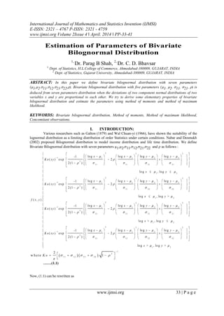
Bivariate Bilognormal distribution with seven parameters 1,2,11,12,21,22 and  as follows :
2 2 2
1 1 1 2 2
2
11 11 21 21
log log log log-1
( ) exp 2
2(1 )
( , )
x x y y
K o xy
f x y
   

   

            
          
          
1 2
2 2 2
1 1 1 2 2
2
11 11 22 22
log , log
log log log log-1
( ) exp 2
2(1 )
x y
x x y y
K o xy
 
   

   

 
            
          
          
1 2
2 2 2
1 1 1 2 2
2
12 12 21 21
log , log >
log log log log-1
( ) exp 2
2(1 )
x y
x x y y
K o xy
 
   

   


            
          
          
1 2
2 2 2
1 1 1 2 2
2
12 12 22 22
log > , log
log log log log-1
( ) exp 2
2(1 )
x y
x x y y
K o xy
 
   

   


            
          
          
1 2
log > , log >x y 























   
1
2
1 1 1 2 2 1 2 2
2
w h ere 1K o     


    
 
….…(1.1)
Now, (1.1) can be rewritten as

2. Estimation of Parameters of Bivariate Bilognormal Distribution
www.ijmsi.org 34 | P a g e
( , ) , ( , ) A }
1 1 2 1 1 1 2 1 1
( , ) , ( , ) A }
1 1 2 2 1 1 2 2 2( , , , )
1 1 2 1 1 2 2 2 ( , ) , ( , ) A }
1 2 2 1 1 2 2 1 3
( , ) , ( , ) A }
1 2 2 2 1 2 2 2 4
A = ( , )
1 1 1 2 1
w h ere
f
f
f
f
f
z
z z z z
z z z z
z z z z
z z z
z z z z
z z

















1 2 2 2
: 0 , 0 , A = ( , ) : 0 , 0
1 1 2 1 2 1 1 2 1 1 1 2 2
A = ( , ) : 0 , 0 , A = ( , ) : 0 , 0
1 1 2 1 1 2 2 1 1 2 2 23 4
z z z z z z
z z z z z z z z
   
   
   
      
  
 
  
 
 
   
   

 

 
 
and
1 2 1 2
1 1 2 1 1 2 2 2
1 1 2 1 1 2 2 2
lo g lo g lo g lo g
, , an d
x y x y
z z z z
   
   
   
   
   
   
   
110 2 2 2
( , ) = e x p 1 2
1 1 1 2 1 1 1 1 1 2 1 2 121 1 2 1
11 2 2 20
( , ) = e x p 1 2
1 1 1 2 2 1 1 1 1 2 2 2 22
1 1 2 2
11 2 2 20
( , ) = e x p 1 2
1 1 2 2 1 1 2 1 2 2 1 2 12
1 2 2 1
K
f z z z z z z
K
f z z z z z z
K
f z z z z z z
 
 
 
 
 
 
 
    
 
 
    
  

   
   
110 2 2 2
( , ) = e x p 1 2
1 1 2 2 2 1 2 1 2 2 2 2 221 2 2 2
K
f z z z z z z 
 
 
 
  
 
    
 
   
1
2
0 1 1 1 1 2 1 2 2
2
= 1k     


   
 
......( 1.2 )
Bivariate Bilognormal distribution with five parameters 1 2 11 21
, , ,    and
12 1 12 22 2 21
w hen andk k      can be deduced from (1.2) as follows :
( , ) , ( , ) A }1 1 2 1 1 1 2 1 1
( , ) , ( , ) A }1 1 2 2 1 1 2 2 2( , , , )1 1 2 1 1 2 2 2 ( , ) , ( , ) A }1 2 2 1 1 2 2 1 3
( , ) , ( , ) A }1 2 2 2 1 2 2 2 4
f z z z z
f z z z z
f z z z z
f z z z z
f z z z z

 
  


where
   
 
0
0
11 2 2 2
( , ) ex p 1 2
1 1 1 2 1 1 1 1 1 2 1 2 12
1 1 2 1
2
11 2 2 2 1
( , ) ex p 1 2
2 1 1 2 1 1 1 1 1 2 22
1 1 2 2 1 2
0
( , )
3 1 2 2 1
1 1 1
K
f
K
f
K
f
z z z z z z
z
z z z z z
k k
z z
k




 
 


    

    

 
 
 
        
  
      
 
 0
2
11 2 21 1 1 1
ex p 1 2
2 1 2 12
2 1 1 1
2 2
11 2 1 1 1 1 2 1 2 1
( , ) ex p 1 2 .
4 1 2 2 1 2
1 1 1 2 2 1 1 1 2 2
K
f
k k k
z z
z z
k k
z z z z
z z
k k k
 
 

 

   

    
        
  
      
            
    
        

3. Estimation of Parameters of Bivariate Bilognormal Distribution
www.ijmsi.org 35 | P a g e
   
1
2
0 11 21 1 2
2
= 1 1 1k k k  


   
 
1 1 2 1
1 2 2 2
1 2
= , =
z z
z z
k k
.......( 1.3)
In section – 2, we derive elementary properties of Bivariate Bilognormal distribution.
In section 3 & 4, we estimate the parameters by the method of moments and method of M.L.E. respectively.
II. ELEMENTARY PROPERTIES:-
The cumulative distribution function of the Bivariate Bilognormal distribution
BVBILN (1, 2, 11, 12,21, 22, is given by
( , ) , ( , ) A
1 1 1 2 1 1 1 2 1 1
( , ) , ( , ) A
2 1 1 2 2 1 1 2 2 2
( , , , )
1 1 2 1 1 2 2 2 ( , ) , ( , ) A
3 1 2 2 1 1 2 2 1 3
( , ) , ( , ) A
4 1 2 2 2 1 2 2 2 4
F
F
F
F
F
z z z z
z z z z
z z z z
z z z z
z z z z












where
2
2
2 1 1 1
1 1 1 2 1 1 1 2 1 1 1
2
2 2 1 1
2 1 1 2 2 1 1 2 1 2 2 1 1 2 2 1 1
2 1 1 1 2 1 1 2
3 1 2 2 1 1 1 2 1 1 2 2 1 1 2
2
4 1 2
( ) 4 ( )
1
( ) 2 ( )+ 4 C ( )
1
( ) 2 + 2 C (2 ( ) 1)
1 1
(
,
, -
,
,
F C
F C
F C
F
z z
z z z
z z
z z z
z z z z
z z z
z




 
 
 
 
    
 

  


  

 
    
 
 
 
 
 
 
 
 
 
   
   
   
   
 
2
1 1 2 1 1 2 2 1
2 2 1 1 2 1 2 2 1 1 1 1 2 1 1 2 2 1
2
) 2 ( ) 2 C 2 C
1 1
C
z zz z
z z

 

      

     
 
   
    
   
   
2 1 1 2 2 2 1 1
1 2 2 1 1 2 1 1 2 2 1 1
2 2
4 C ( ) + 4 C ( )
1 1
z z z z
z z
 
   
 
    
       
       
......
( 2.1 )
C-1 = (11 + 12) (21 + 22) and  (.) denotes the cumulative distribution function of the standard normal
distribution. The cumulative distribution function of BVBILN (1, 2, 11, 21, can be deduced from
(2.1) as follows :
1 1 1 2 1 1 1 2 1 1
2 1 1 2 1 1 1 2 1 2
1 1 2 1
3 1 2 2 1 1 2 2 1 3
4 1 2 2 1 1 2 2 1 4
( ) , ( ) A
( ) , ( ) A
( )
( ) , ( ) A
( ) , ( ) A
, ,
, ,
,
, ,
, ,
F
F
F
F
F
z z z z
z z z z
z z
z z z z
z z z z












........ ( 2.2 )
where

4. Estimation of Parameters of Bivariate Bilognormal Distribution
www.ijmsi.org 36 | P a g e
 2
2 1 1 1
1 1 1 2 1 1 1
2 1
1 1
2
2 1 1 2 1 2 1 1
2
1 1
2 1
2 1 1 1 1 1 1
3 1 2 2 1 1 1 2
2
1
4 1 2 2 1
*
2
*
* *
2
*
( ) 4
1
( ) 2 (1 ) 4
1
( ) 2 ( ) 4
1
( )
1
, ( )
,
, 1
,
F C
F C k C k
F C C
F
z
k
z z
z z z
z
z z z
z
z
z z z k
z z k k k
k
z z




 


  


    

    



 
 
 
 
 
 
 
 
 
 
 
    
          
 
 
 
1 1
2 1
1 1 2 1 1
2 1 1 1
2 2
1 1 2 1
2 1 1 1
1 1 1 2
1 2 1 1
2 2
1
*
* *
*
2 (1 ) ( ) 2
1 1
4 4
1 1
C C
C C
z
z
z z k
k z k
z z
z z
z k k
k k z
k
 


 
 

     
 
     
 
  
  
    
 
 
   
 
   
 
   
 
      
   
   
where   1 1 1
* 1 2
k kC
   
11 21
  and  (.) denotes the cumulative distribution function of the
standard normal distribution.
Note that it is easy to simulate observations with density (1.1).
If we define z
1
and z
2
as standard normal variables & define
 
1 2
1 2
1 2
1 2
1 1 1 2 2 1
2 1 1 2 2 2
1 1 2 2 2 1
1
w ith p ro b ab ility
1
w ith p ro b ab ility
2
w ith p ro b ab ility
3
,
,
,
,
z z
e e
z z
e e
z z
z z
e e
e
   
   
   
 



 
 
 

 
 
 
 
 
 

 
 
 
1 21 2 2 2 2
w ith p ro b ab ility
4
,
z z
e
 












  
  
  
…...(2.3)
where

5. Estimation of Parameters of Bivariate Bilognormal Distribution
www.ijmsi.org 37 | P a g e
 
   
 
   
 
   
 
   
1 1 2 1
1 1 1 2 2 1 2 2
1 1 1 2 2 1 2 2
1 2 2 1
1 1 1 2 2 1 2 2
1 2 2 2
1 2
1 1 2 1 2 2
1 2
1 2
1 2
P r o b lo g , lo g
1
1 1 2 2
P r o b lo g , lo g
2
P ro b lo g , lo g =
3
P ro b lo g , lo g
4
1 2
x y
x y
x y
x y
 
  
   
 
  
   
 
  
   
 
  
   
   
 
   
 
  
 
   
 
........ (2.4)
then (x, y) has the BVBILN (1, 2, 11, 12, 21, 22, distribution. Note that if we define (z1, z2) as
 
2 2 1
1 2
1 2
1 2
1 2
1 1 1 2 2 1
1 1 1 2 2 2 1
1 1 1 1
w ith p ro b ab ility
1
w ith p ro b ab ility
2
w ith p ro b ab ili
,
,
,
,
k
k
z z
e e
z z
e e
z z
z z
e e
 
   
   
 



 
 

 
 
 
 
 
 

 
 
 
2 2 2 11 21 1 1 1
ty
3
w ith p ro b ab ility
4
,
kk z z
e e
  













  
  
  
where   1
1 1
1 1 2
k k

   ,   1
1 1
2 1 2 2
/k k k

   ,
  1
1 1
3 1 2 1
/k k k

   and   1
1 1
4 1 2 1 2
/k k k k

  
....... (2.5)
then (x, y) has the BVBILN (1, 2, 11, 21, distribution.
The tth row moments of BVBILN (1, 2, 11, 21, distribution about zero are given by
 '
0
r
E x
r 
 
    
1 1 1
1 1 1 1 1
1
2 21 12 2
2 1 12 2 1
11
r r re
e r k e k r
k
  
 
 
 
       
  
 
........(2.6)
and
 '
0
t
E y
s 
 
    
2
2
1
2
2
2 1
2 22 2
2 1 2 1
2
2
2
1
2 1 2
1
1
2
s
e
e e
k
k
s s k
s k s


 
     


 
 
 
 
 
....(2.7)
The moments of (log x, log y) about (1, 2) are given by

6. Estimation of Parameters of Bivariate Bilognormal Distribution
www.ijmsi.org 38 | P a g e
 
 
 
  1
1
2 1
0
1 1*
1
1
2 2
lo g 1
1
r
r
r
r
r r
r
E x
k
k






    

 
 
 
....(2.8)
 
 
 
  2
2
0
2
* 2 1
2
1
1
2 2
lo g 1
1
s
ss
s
s
r
E y
k
s
k






    

 
 
 
....(2.9)
Putting r = 1, 2, 3,…. in (2.8) and (2.9) we get
   1 11 1
*
1 0
2
= E lo g - = 1 ,x k 

 
   
2
1 1 1
2
11
* 2
20
= E log - = 1x k k   
     1 1
3
1
3
1 1
* 2
3 0
2
= E lo g - = 2 1 1x k k

  
   2 2 1 20 1
2
= E lo g = 1* y k 

  
   
2
2
2
02 21 2 2
2
= E log - = 1* x k k   
     
3 3
0 3 2 2 1 2 2
22
= E lo g - = 2 1 1* y k k

   
The central moments of log x and log y of order two and three are given by
 
2
* *
2 0 1 0
2 0
   
 
2
1 1 11
22
(1 )1( ) kk

  
* * * *3
3 2
3 0 3 0 2 0 1 0 1 0
      
    
3
11 1 1
2
1
2 4
1 ( 1) 1
1
k kk k



    
 
  
and
 
2
0 1
* *
0 2 0 2
  
 2
2 1
2
2
2 2
1( 1) kk

 
 
  
* * * *3
3 2
0 3 0 3 0 2 0 1 0 1
      
     
2
2 2 2 2
3
2 1
2 4
1 1 1k k k k
 
    
 
  
III. ESTIMATION BY THE METHOD OF MOMENTS:-
It is difficult to obtain the estimators of the parameters 1, 2, 11, 21, and  using the row moments
of (x, y) given in (2.6) and (2.7). If 11, 21, and  are known, then the estimators of 1, 2, based on
moments of (x, y) are given by:

7. Estimation of Parameters of Bivariate Bilognormal Distribution
www.ijmsi.org 39 | P a g e
  
    
2 2 2
1 1 1 1 1
1 1 0
1 1 1
2 2
1 1 1 1 1 1
1 +
= lo g
2 1
k
k m
e k e k
 

 
 
 
 
 
  
       
  
........(3.1)
and
  
    
2 0 1
2
2 1 2 2 1
2
2 1
2 2
2 2 1
1
2
2
1 +
= lo g
2 1
1
2
k m
e e
k
kk






     
 
 
 
 
   
  
   
..........(3.2)
where 1 0
1
1
=
n
n
i
i
m x

  0 1
1
1
an d =
n
n
i
i
m y

 
However these estimators are found to be less efficient then the estimators based on the moments of
(Log x, Log y), namely.
2
= - ( 1)
1 10 11 1
m k 


and
2
= - ( 1)
2 01 21 2
m k 


..........(3.3)
where
1 0
1
1
= lo g
n
n
i
i
m x


n
0 1
i= 1
1
an d = lo g
n
i
m y
It can be observed that
 
 1 2
,  is not satisfactory when ,
12 11 22 21
     . Hence to estimate the
parameters 1, 2, 11, 21, and  the following method is adopted. Denote the sample mean of (log xi,
log yi ) (i = 1,2,3,4........n) by ( 1 0
m , 0 1
m ) and central sample moments of order two and three by ( 2 0
m , 0 2
m )
and ( 3 0
m , 0 3
m ) respectively. Then the moment estimates satisfy the equations:-
 
 
 
 
2
= + ( 1 )
1 0 1 1 1 1
2
= + ( 1 )
1 0 2 2 1 2
222 2
= 1 1 +
2 0 1 1 1 1 1 1
222 2
= 1 1 +
0 2 2 1 2 2 2 1
22 43
= ( 1 ) 1 1 +
3 0 1 1 1 1 1
3 22 4
= ( 1 ) 1 1 +
0 3 2 1 2 2 2
m k
m k
m k k
m k k
m k k k
m k k k
 

 

 

 


 

 


 
  
 
 
  
 
  
    
  

 
   
 





8. Estimation of Parameters of Bivariate Bilognormal Distribution
www.ijmsi.org 40 | P a g e
The above equations are solved by the procedure given by John(1982) subject to the conditions.
3 1
2 2
3 3
2 2
3
2
3 0 2 0 0 3 0 2
1
2= < 1 1 & = < 1 1
2 2 2 2
m m m m
           
            
       
The moment estimators are given by
2
2
= B , B = 1
1 1 0 1 1 1 1 12
= B , B = 1
2 0 1 2 2 2 1 22
2B B 4 B B 4
1 1 1 2 2
= , =
1 1 2 12 2
m k
m k
C C


 
 
 
 
  
 
 
 
 
 
 
   
 
 
 
and
2 2
B 4 B B 4 B
1 1 1 2 2 22 2
= , =
1 2 2 22 2
2 2
= + B 4 B 4
1 2 1 1 2 2
2 2
= , =
1 1 1 1 2 2 1 1
C C
B B C C
C k C k 
 

   
 
 
 

IV. ESTIMATION BY THE METHOD OF M.L.E:-
Let (x
[1:n]
, y
[1:n]
), (x
[1:n]
, y
[2:n]
),...,(x[n:n], y[n:n]) be a random sample of concomitant ordered paired
observations of size n from BVBILN (1, 2, 11, 21, . The likelihood function is given by
Log L = Const. - n(log11 + log21 + 1/2log(1 - 2))
   1 1 2 1 1 1 2 1
1 2
2 2 2
2 2 2 211 11 21 21 11 21 21
11 21 11 21 2
1 1 2
1
2 2 2
3 4
21
2
21
2
2
2 21
2 2
2 (1 )
z
k
z
z z z z z
z z z z z z
z z z
k k k
kk k

 

 
           

     
       
   
     

.…….(4.1)
where Const. =    
4
2
lo g lo g 1 lo g 1 lo g lo g
1 2
1
n k k x y
i i i
      
            
       
,
Z11 = 1 2
2 1
1 1 2 1
(lo g ) (lo g )
an d Z
x x 
 
 
 Note that , , ,
2 3 4I
    denotes the summation over all
observations such that the conditions (i) log x  1, log y  2 (ii) log x  1, log y > 2, (iii) log x > 1, log
y  2 and (iv) log x  1, log y  2 are satisfied by the n concomitant ordered paired observations
respectively. The likelihood equations are given by
 
lo g 1 2 1 1 1 2 1 1 1 2 1
0 0
1 1 2 1 1 1 2 2
1 2 3 41 1 1 2 1 21 1 1
Z Z Z Z ZL
Z Z Z
k k kk k k
 
 
 
     
                    
            
… ....(4.2)
 
lo g 1 2 1 1 1 1 1 2 1 1 1
0 0
2 1 1 1 2 12 2
1 2 3 42 2 1 2 1 22 1 2
Z Z Z Z ZL
Z Z Z
k k kk k k
 
 
 
      
                     
             
....(4.3)

9. Estimation of Parameters of Bivariate Bilognormal Distribution
www.ijmsi.org 41 | P a g e
Solving (4.2) and (4.3) for 1 and 2 we get
   
2 lo g lo g lo g lo g
1
1 2 3 4^
1 2
1 1 2 3 4
x x x xk
r r r rk

  
        
   

  
…...(4.4)
and
   
2 lo g lo g lo g lo g
2
1 3 2 4^
2 2
2 1 3 2 4
y y y yk
r r r rk

   
         
  

  
….(4.5)
where r1, r2, r3 and r4 are the numbers of paired ordered observations satisfied the conditions (i) logx 1,
logy 2, (ii) logx 1, logy > 2, (iii) logx >1, logy 2, and (iv) logx > 1, logy > 2 respectively with
4
1
r n
i
i


. Further by differentiating (4.1) with respect to 11, 21 and and equating them to zero and
solving them simultaneously we get
       
2 2 2 2
2 lo g lo g lo g lo g
1 1 1 1 12 1 2 3 4
^ 21 1
1
x x x xk
n k
   

      
              
       

 
 
 
 
....(4.6)
       
2 2 2 2
2 lo g lo g lo g lo g
2 2 2 22 1 3 2 4
^ 22 1
2
y y y yk
n k
   

       
              
     

 
 
 
 
....(4.7)
and
               1 2 1 2 1 1 2 2 1 2 1 2
1
^ ^
1 2 11 21
2 3 4^
log log log log log log log logk k x y k x y k x y x y
nk k
       

 
           

  
.…(4.8)
REFERENCES
[1]. Garvin, J. S. and McClean, S.L.(1997). Convolution and sampling theory of the binormal distribution as a prerequisite to its
application in statistical process control. The Statistician, 46, No. 1, pp 33-47.
[2]. H.N. Nagaraja (2005). Function of Conconitants of order statistics - ISPS Vol. 7, 16-32.
[3]. John, S. (1982). The three-parameter two-piece normal family of distribution and its fitting. Commun. Statist. – Theor and
Meth, 11, 879-885.
[4]. Kimber, A.C. (1985) Methods for the two-piece normal distribution. Commun. Statist. – Theor. And Meth, 14(1), 235-245.
[5]. S. P. Nabar and S. C. Deshmukh. (2002) On Estimation of Parameters of Bilognormal Distribution. Journal of the Indian
Statistical Association Vol. 40, 1, 2002, 59-70.
[6]. S.P. Nabar & S.P.Parpande (2001) A note on the maximum likelihood estimator of the binormal distribution BIN (, , ).