The document discusses reduced row-echelon matrices and provides examples of elementary row operations used to transform matrices into reduced row-echelon form. It gives the initial matrix, shows the elementary row operations used, and provides the resulting reduced row-echelon matrix. Several examples are provided with the goal of getting a 1 in the upper left corner and clearing out the rest of the first column through row operations.

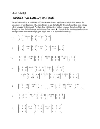
1. SECTION 3.3
REDUCED ROW-ECHELON MATRICES
Each of the matrices in Problems 1-20 can be transformed to reduced echelon form without the
appearance of any fractions. The main thing is to get started right. Generally our first goal is to get
a 1 in the upper left corner of A, then clear out the rest of the first column. In each problem we
first give at least the initial steps, and then the final result E. The particular sequence of elementary
row operations used is not unique; you might find E in a quite different way.
1 2  R 2−3 R1 1 2  R1− 2 R 2 1 0
1. 3 7  → 0 1  → 0 1 
     
3 7  R1− R 2 1 2  R 2− 2 R1 1 2  R1− 2 R 2 1 0 
2. 2 5  → 2 5  → 0 1  → 0 1 
       
 3 7 15 R1− R 2 1 2 4  R 2− 2 R1 1 2 4  R1− 2 R 2 1 0 2 
3.  2 5 11 →  2 5 11 → 0 1 3  → 0 1 3 
       
3 7 −1 R 2− R1  3 7 −1 R1− R 2 1 12 −10 
4. 5 2 8  →  2 −5 9  →  2 −5 9 
     
R 2− 2 R1 1 12 −10  ( −1/ 29) R 2 1 12 −10  R1−12 R 2 1 0 2 
→ 0 −29 29  → 0 1 −1  → 0 1 −1
     
1 2 −11 R 2− 2 R1 1 2 −11 ( −1) R 2 1 2 −11 R1− 2 R 2  1 0 −5 
5.  2 3 −19  →  0 −1 3  →  0 1 −3  →  0 1 −3 
       
1 −2 19  R 2− 4 R1 1 −2 19  R1+ 2 R 2 1 0 7 
6.  4 −7 70  →  0 1 −6  → 0 1 −6 
     
1 2 3 1 2 3  1 2 3 
R 2− R1 R 3− 2 R1
7. 1 4 1  →  0 2 −2  →  0 2 −2 
     
2 1 9 
  2 1 9 
  0 −3 3 
 

2. 1 2 3  1 2 3  1 0 5 
(1/ 2) R 2 R 3+3 R 2 R1− 2 R 2
→  0 1 −1 →  0 1 −1 →  0 1 −1
     
 0 −3 3 
  0 0 0 
  0 0 0 
 
1 −4 −5  1 −4 −5   1 −4 −5 
R 2−3 R1 R3− R1
8. 3 −9 3  → 0 3 18  → 0 3 18 
     

1 −2 3 
  1 −2 3 
  0 2 8 
 
 1 −4 − 5   1 −4 −5  ( −1/12) R 3
1 0 0
R 2− R 3 R 3− 2 R 2
→  0 1 10  →  0 1 10  → → 0 1 0
     
0 2 8 
   0 0 −12
  0 0 1
 
 5 2 18 1 1 6  1 1 6 
R1− R 3 R 3− 4 R1
9. 0 1 4  → 0 1 4  → 0 1 4 
     
 4 1 12
   4 1 12 
  0 −3 −12 
 
1 1 6  1 0 2 
R 3+3 R 2 R1− R 2
→ 0 1 4  → 0 1 4 
   
0 0 0 
  0 0 0 
 
 5 2 −5  1 1 2  1 1 2 
R1− R 3 R 2−9 R1
10.  9 4 −7  →  9 4 −7  →  0 −5 −25
     
 4 1 −7 
   4 1 −7 
   4 1 −7 
 
1 1 2 
( −1/5) R 2
1 1 2   1 0 − 3
R 3−4 R1 R 3+3 R 2
→ 0 −5 −25  → 0 1 5  → → 0 1 5 
     
0 −3 −15 
  0 −3 −15
  0 0 0 
 
3 9 1   1 3 −6   1 3 −6 
SWAP ( R1, R 3) R 2− 2 R1
11. 2 6 7  → 2 6 7  →  0 0 19 
     
 1 3 −6 
  3 9 1 
  3 9 1 
 
 1 3 −6   1 3 −6  1 3 0
R 3−3 R1 (1/19) R 2 R 3−19 R 2
→ 0 0 19  → 0 0 1  → 0 0 1 
     
0 0 19 
  0 0 19 
  0 0 0
 

3.  1 −4 −2  R 2−3 R1
 1 −4 −2  R3− 2 R1
 1 −4 −2 
12.  3 −12 1  → 0 0 7  → 0 0 7 
     
 2 −8 5 
   2 −8 5 
  0 0 9 
 
(1/7) R 2
 1 −4 0 
→ → 0 0 1
 
0 0 0
 
2 7 4 0  SWAP ( R1, R 2)
1 3 2 1  R 2− 2 R1
1 3 2 1 
13. 1 3 2 1  → 2 7 4 0 →  0 1 0 −2 
     
2 6 5 4 
  2 6 5 4
  2 6 5 4 
 
R 2− 2 R1
1 3 2 1  R1−3 R 2
1 0 0 3 
→  0 1 0 −2  → →  0 1 0 −2 
   
0 0 1 2 
  0 0 1 2 
 
1 3 2 5  R 2− 2 R1
1 3 2 5  R 3−2 R1
1 3 2 5 
14. 2 5 2 3  →  0 −1 −2 −7  →  0 −1 −2 −7 
     
 2 7 7 22 
   2 7 7 22 
   0 1 3 12 
 
R 3+ R 2
1 3 2 5  ( −1) R 2
1 0 0 4 
→ 0 −1 −2 −7  → →  0 1 0 − 3
   
0 0 1
 5  0 0 1 5 
 
2 2 4 2  SWAP ( R1,R 2)
 1 −1 −4 3  R 2− 2 R1
 1 −1 −4 3 
15.  1 −1 −4 3  → 2 2 4 2  → 0 4 12 −4 
     
 2 7 19 −3
   2 7 19 −3
   2 7 19 −3
 
R 3−2 R1
 1 −1 −4 3  (1/ 4) R 2
 1 − 1 −4 3 
→ 0 4 12 −4 →  0 1 3 − 1
   
0 9 27 −9 
  0 9 27 −9 
 
R 3−9 R 2
 1 −1 −4 3   1 0 −1 2 
R1+ R 2
→ 0 1 3 −1 → 0 1 3 −1
   
0 0 0 0 
  0 0 0 0 
 

4. 1 3 15 7  R 2− 2 R1
1 3 15 7  R 3−2 R1
1 3 15 7 
16.  2 4 22 8  →  0 −2 −8 −6  →  0 −2 −8 −6 
     
 2 7 34 17 
   2 7 34 17 
  0 1 4 3 
 
( −1/ 2) R 2
1 3 15 7   1 0 3 −2 
R 3− R 2
→ 0 1 4 3 → → 0 1 4 3 
   
0 1 4 3
  0 0 0 0 
 
 1 1 1 −1 −4   1 1 1 −1 −4  R 3−2 R1
1 1 1 −1 −4 
R 2− R1
17. 1 −2 −2 8 −1 →  0 −3 −3 9 3  →  0 −3 −3 9 3 
     
 2 3 −1 3 11 
   2 3 −1 3 11 
  0 1 −3 5 19 
 
( −1/3) R 2
1 1 1 −1 −4  1 1 1 −1 −4 
R 3− R 2
→ 0 1 1 −3 −1 → 0 1 1 −3 −1
   
0 1 −3 5 19 
  0 0 −4 8 20 
 
( −1/ 4) R 3
1 1 1 −1 −4   1 0 0 2 −3 
R1− R 2
→ 0 1 1 −3 −1 → →  0 1 0 −1 4 
   
 0 0 1 −2 −5 
  0 0 1 −2 −5
 
1 −2 −5 −12 1  1 −2 −5 −12 1  R 3−2 R1 1 −2 −5 −12 1 
−2
18.  2 3 18 11 9  R 2→R1  0 7 28 35 7  → 0 7 28 35 7 
     
 2 5 26 21 11
   2 5 26 21 11
  0 9 36 45 9 
 
1 −2 −5 −12 1 
(1/7) R 2 (1/7) R 2
1 −2 −5 −12 1 
→ 0 1 4
 5 1  → 0 1 4
 5 1 
0 9 36 45 9 
  0 9 36 45 9 
 
1 −2 −5 −12 1  1 0 3 −2 3 
(1/9) R 3 R 3− R 2
→ 0 1 4 5 1 → → 0 1 4 5 1 
   
0 1 4
 5 1 0 0 0 0 0 
 
 2 7 −10 −19 13 SWAP ( R1, R 3)
1 0 2 1 3
19.  1 3 −4 −8 6  →  1 3 −4 −8 6 
   
1 0 2
 1 
3  2 7 −10 −19 13
 

5. 1 0 2 1 3
R 3−2 R1
1 0 2 1 3
R 2− R1
→  0 3 −6 −9 3  →  0 3 −6 −9 3 
   
 2 7 −10 −19 13
  0 7 −14 −21 7 
 
(1/3) R 2
1 0 2 1 3
R 3−7 R 2
1 0 2 1 3 
→  0 1 −2 −3 1  →  0 1 −2 − 3 1 
   
0 7 −14 −21 7 
  0 0 0 0 0
 
 3 6 1 7 13  1 2 −4 −2 −13
R1− R 3
20.  5 10 8 18 47  →  5 10 8 18 47 
   
 2 4 5 9 26 
   2 4 5 9 26 
 
1 2 −4 −2 −13 1 2 −4 −2 −13
R 2−5 R1 R 3− 2 R1
→  0 0 28 28 112  → 0 0 28 28 112 
   
 2 4 5 9 26 
  0 0 13 13 52 
 
(1/ 28) R 2
1 2 −4 −2 −13 R 3−13 R 2
1 2 0 2 3 
→ 0 0 1 1 4  → → 0 0 1 1 4 
   
0 0 13 13 52 
  0 0 0 0 0 
 
In each of Problems 21-30, we give just the first two or three steps in the reduction. Then we
display the resulting reduced echelon form E of the augmented coefficient matrix A of the
given linear system, and finally list the resulting solution (if any).
21. Begin by interchanging rows 1 and 2 of A. Then subtract twice row 1 both from row 2
and from row 3.
1 0 0 3 
E =  0 1 0 −2  ;
  x1 = 3, x2 = −2, x3 = 4
0 0 1 4 
 
22. Begin by subtracting row 2 of A from row 1. Then subtract twice row 1 both from row
2 and from row 3.
1 0 0 5 
E = 0 1 0 −3 ;
  x1 = 5, x2 = −3, x3 = 2
0 0 1 2 
 

6. 23. Begin by subtracting twice row 1 of A both from row 2 and from row 3. Then add row
2 to row 3.
1 0 −3 14 
E = 0 1 2 3  ;
  x1 = 4 + 3t , x2 = 3 − 2t , x3 = t
0 0 0 0 
 
24. Begin by interchanging rows 1 and 3 of A. Then subtract twice row 1 from row 2, and
three times row 1 from row 3.
1 −2 0 5 
E = 0 0 1 7  ;
  x1 = 5 + 2t , x2 = t , x3 = 7
0 0 0 0 
 
25. Begin by interchanging rows 1 and 2 of A. Then subtract three times row 1 from row 2,
and five times row 1 from row 3.
1 0 −2 0 
E = 0 1 3 0  .
  The system has no solution.
0 0 0 1 
 
26. Begin by subtracting row 1 from row 2 of A. Then interchange rows 1 and 2. Next
subtract twice row 1 from row 2, and five times row 1 from row 3.
1 0 1 0 
E = 0 1 2 0  .
  The system has no solution.
0 0 0 1 
 
27. x1 − 4 x2 − 3 x3 − 3 x4 = 4
2 x1 − 6 x2 − 5 x3 − 5 x4 = 5
3x1 − x2 − 4 x3 − 5 x4 = − 7
[The first printing of the textbook had a misprinted 2 (instead of 4) as the right-hand
side constant in the first equation.] Begin by subtracting twice row 1 from row 2 of A,
and three times row 1 from row 3.
1 0 0 2 3 
E = 0 1 0 −1 −4  ;
  x1 = 3 − 2t , x2 = −4 + t , x3 = 5 − 3t , x4 = t
0 0 1 3 5 
 

7. 28. Begin by subtracting row 3 from row 1 of A. Then subtract 3 times row 1 from row 2,
and twice row 1 from row 3.
 1 −2 0 3 4 
E = 0 0 1 4 3  ;
  x1 = 4 + 2 s − 3t , x2 = s, x3 = 3 − 4t , x4 = t
0 0 0 0 0 
 
29. Begin by interchanging rows 1 and 2 of A. Then subtract three times row 1 from row 2,
and four times row 1 from row 3.
1 0 1 1 3 
E =  0 1 −2 3 5  ;
  x1 = 3 − s − t , x2 = 5 + 2s − 3t , x3 = s, x4 = t
0 0 0 0 0 
 
30. Begin by interchanging rows 1 and 2 of A. Then subtract twice row 1 from row 2, and
five times row 1 from row 3.
 1 0 0 0 −3 2 
E =  0 1 0 −1 2 1  ;
  x1 = 2 + 3t , x2 = 1 + s − 2t , x3 = 2 + 2s, x4 = s, x5 = t
 0 0 1 −2 0 2 
 
1 2 3  (1/6) R3
 1 2 3 R 2−5 R 3
1 2 3  (1/ 4) R 2
1 2 3 
31. 0 4 5  → 0 4 5 → 0 4 0  → 0 1 0 
       
0 0 6 
  0 0 1
  0 0 1 
  0 0 1 
 
1 0 3  1 0 0 
R1−2 R 2 R1−3 R 3
→ 0 1 0  → 0 1 0 
   
0 0 1 
  0 0 1 
 
32. If ad − bc ≠ 0, then not both a and b can be zero. If, for instance, a ≠ 0, then
a b  (1/ a ) R1 1 b / a  R 2−c R1 1 b / a  a R 2 1 b/a 
c d  → c d  → 0 d − bc / a  → 0 ad − bc 
       
(1/( ad −bc )) R 2 1 b / a  R1−(b / a ) R 2 1 0 
→ 0 1  → 0 1  .
   
33. If the upper left element of a 2 × 2 reduced echelon matrix is 1, then the possibilities are
1 0  1 * 
0 1  and 0 0  , depending on whether there is a nonzero element in the second
   

8. row. If the upper left element is zero — so both elements of the second row are also 0,
0 1  0 0 
then the possibilities are   and 0 0  .
0 0   
34. If the upper left element of a 3 × 3 reduced echelon matrix is 1, then the possibilities are
1 0 0  1 0 *  1 * 0  1 * * 
0 1 0  , 0 1 *  , 0 0 1  , and 0 0 0  ,
       
0 0 1 
  0 0 0 
  0 0 0
  0 0 0 
 
depending on whether the second and third row contain any nonzero elements. If the
upper left element is zero — so the first column and third row contain no nonzero
elements — then use of the four 2 × 2 reduced echelon matrices of Problem 33 (for the
upper right 2 × 2 submatrix of our reduced 3 × 3 matrix) gives the additional possibilities
0 1 0  0 1 *  0 0 1  0 0 0 
0 0 1  , 0 0 0  , 0 0 0  , and 0 0 0  .
       
0 0 0 
  0 0 0 
  0 0 0 
  0 0 0 
 
35. (a) If ( x0 , y0 ) is a solution, then it follows that
a (kx0 ) + b(ky0 ) = k (ax0 + by0 ) = k ⋅ 0 = 0,
c( kx0 ) + d ( ky0 ) = k (cx0 + dy0 ) = k ⋅ 0 = 0
so (kx0 , ky0 ) is also a solution.
(b) If ( x1 , y1 ) and ( x2 , y2 ) are solutions, then it follows that
a ( x1 + x2 ) + b( y1 + y2 ) = (ax1 + by1 ) + (ax2 + by2 ) = 0 + 0 = 0,
c( x1 + x2 ) + d ( y1 + y2 ) = (cx1 + dy1 ) + (cx2 + dy2 ) = 0 + 0 = 0
so ( x1 + x2 , y1 + y2 ) is also a solution.
36. By Problem 32, the coefficient matrix of the given homogeneous 2 × 2 system is row-
equivalent to the 2 × 2 identity matrix. Therefore, Theorem 4 implies that the given
system has only the trivial solution.
37. If ad − bc = 0 then, much as in Problem 32, we see that the second row of the reduced
echelon form of the coefficient matrix is allzero. Hence there is a free variable, and thus
the given homogeneous system has a nontrivial solution involving a parameter t.

9. 38. By Problem 37, there is a nontrivial solution if and only if
(c + 2)(c − 3) − (2)(3) = c 2 − c − 12 = (c − 4)(c + 3) = 0,
that is, either c = 4 or c = –3.
39. It is given that the augmented coefficient matrix of the homogeneous 3 × 3 system has the
form
 a1 b1 c1 0
 a b2 c2 0 .
 2 
 pa1 + qa2 pb1 + qb2 pc1 + qc2 0 
 
Upon subtracting both p times row 1 and q times row 2 from row 3, we get the matrix
 a1 b1 c1 0
a b2 c2 0
 2 
0
 0 0 0

corresponding to two homogeneous linear equations in three unknowns. Hence there is at
least one free variable, and thus the system has a nontrivial family of solutions.
40. In reducing further from the echelon matrix E to the matrix E*, the leading entries of
E become the leading ones in the reduced echelon matrix E*. Thus the nonzero rows of
E* come precisely from the nonzero rows of E. We therefore are talking about the same
rows — and in particular about the same number of rows — in either case.