3D Curve Project

Computer Graphics January 12,2007
1
Report of 3D curve project
Chunhui Chen Mat. 123721
Email: njucch@hotmail.com
University of Trento, Department of Computer Science
Abstract
Java3D is an Application Programming Interface used for writing 3D graphics applications and
applets. This paper gives a short introduction of java3D, analyses the mathematics of Hermite,
Bezier, FourPoints, B-Splines curve, and describes implementation of curve creation and curve
operations using Java3D API.
Keywords:
Java3D, curve, Hermite, Bezier, FourPoints, B-Splines
1. Java3D Introduction
The Java 3D API is an interface for writing programs to display and interact with
three-dimensional graphics. The API provides a collection of high-level constructs for creating
and manipulating 3D geometry and structures for rendering that geometry. Java 3D provides the
functions for creation of imagery, visualizations, animations, and interactive 3D graphics
application programs.
A Java 3D application builds and manipulates a scene graph by constructing Java 3D objects and
then later modifying those objects by using their methods. A Java 3D program first constructs a
scene graph, once built, hands that scene graph to Java 3D for processing. The structure of a scene
graph is Directed Acyclic Graph (DAG), parent-child relationship, and tree structure with root,
branch and leaf.

2
2. Curve Mathematics
All curve design is concerned with the creation of smooth curves based on a small number of
user-controlled parameters. It is common that the curve has two endpoints and other controls to
vary the shape of the curve. Cubic polynomials are very popular in curve design.
Complex curves are often created segment-by-segment, using simpler curves for each segment.
Therefore, the complete curve is determined by each segment and the continuity conditions at
each join point.
Geometric Continuity:
G0: Curves are joined
G1: First derivatives are proportional at the join point. The curve tangents have the same
direction, but not necessarily the same magnitude.
G2: First and second derivatives are proportional at the join point.
Parametric Continuity:
C0: Curves are joined.
C1: First derivatives are equal.
C2: First and second derivatives are equal.
Cn: The nth derivatives are equal.
Many curve are defined on a parameter t. Instead of the function y=f(x), the curve is defined as
x=f(t), y=g(t), z=s(t), tε[0,1]. One popular method is to describe the curve as a matrix equation
involving a basis matrix M, a geometry vector g, and a polynomial vector p.
The general form for a parametric curve can be written as:
Mgpt t
k=)(θ
The blending function is represented by Mpt
k , which give the curve its unique shape. The basis
matrix M determines the coefficients of the blending function. The geometric constraints are
multiplied by blending function. It is common thus to differentiate different types of curves based
on geometric constraints and the basis matrix.
Hermite Curves
Hermite curves are a foundation of interactive curve design. Commonly hermite curves are
designed by two control points and tangent segments at each control point. Tangent handles may
be interactively changed to adjust the shape of the curve once control points are placed. Hermite
curves are easy to implement but have a number of drawbacks. For instance, it is difficult to
determine how long to make a tangent handle in order to create a desired shape.
To calculate a Hermite curve, we need the following vectors:

3
0P : The startpoint of the curve
0T : The tangent vector at the first point (how the curve leaves the start point).
1P : The endpoint of the curve
1T : The tangent vector at the endpoint.
The geometric constraints can be written in the form,
t
TTPPg ],,,[ 1010=
Here we consider only x-component of the Hermite curve, as y and z components are the same.
Mgttttx )1,,,()( 23
=
The required equations are x (0), x (1), )0('
x , )1('
x
Mgx t
]1,0,0,0[)0( =
Mgx t
]1,1,1,1[)1( =
Since Mgtttx t
]0,1,2,3[)( 2'
=
Mgx t
]0,1,0,0[)0('
=
Mgx t
]0,1,2,3[)1('
=
Assume
t
xxxxg )]1(),0(),1(),0([ ''*
= ,
**
0123
0100
1111
1000
Mgg
⎥
⎥
⎥
⎥
⎦
⎤
⎢
⎢
⎢
⎢
⎣
⎡
=
Calculate inversion of matrix, we can get M as:
⎥
⎥
⎥
⎥
⎦
⎤
⎢
⎢
⎢
⎢
⎣
⎡
−−−
−
=
0001
0100
1233
1122
M
This yields blending function as:
132)( 23
1 +−= tttb

4
23
2 32)( tttb +−=
ttttb +−= 23
3 2)(
23
4 )( tttb −=
Thus,
14031201 )()()()()( TtbTtbPtbPtbt +++=θ
Drawing a single segment of a Hermite curve is relatively straightforward. A more complex shape
can be created with piecewise Hermite curve segments. It is necessary to decide the continuity at
the join point. In fact, it is not easy to construct desired shapes for a single segment as the tangent
handles have to be moved very far away from the control points to produce significant bends. It is
a drawback of Hermite curves. A possible method for this drawback is to weight the blending
functions for the tangent vector. Or it is possible to relax the need for tangent handles by
converting a Hermite curve into a cardinal spline.
Bezier Curve
As discussed above, using tangent handles to adjust the shape of curve is somewhat clumsy. The
difficulties increase when creating piecewise cubic Hermite curves. Compensating for these
drawbacks leads into Bezier curves.
Linear Bezier
Linear Bezier curve is obtained by linear interpolation between two control points 0P , 1P ;
10)1()( tPPtt +−=θ , ]1,0[∈t
Quadratic Bezier
Quadratic Bezier is obtained by deCasteljau algorithm as a linear interpolation between linear
interpolation between control points 0P , 1P , 2P .
Consider three control points, on the line segment 0P 1P , point
)1(
1P in the ratio (1-t): t. The
point
)1(
2P on the segment 1P 2P is at the same ratio. Then draw a line from
)1(
1P to
)1(
2P .
Locate the point )(tθ at the same ratio on that line segment. This is the point on the curve at the
specified value of t, ]1,0[∈t . As show below:

5
])1[(])1)[(1()1()( 2110
)1(
2
)1(
1 tPPtttPPtttPPtt +−++−−=+−=θ
2
2
10
2
)1(2)1()( PtPttPtt +−+−=θ
With Bezier curves, tangents are implicitly specified. The geometric constraints are the individual
control points. The blending functions are as below:
2
0 )1()( ttb −=
)1(2)(1 tttb −=
2
2 )( ttb =
These blending functions happen to be the second-order Bernstein polynomials. In fact, it can be
extended that higher-order Bezier curves use higher-order Bernstein polynomials as their blending
functions.
Bernstein polynomials is defined by
ini
ni tt
iin
n
tB −
−
−
= )1(
!)!(
!
)(,
Cubic Bezier
Bezier curves are described as one method for implicitly specifying tangents. The tangent is
simply the vector created from segments extending from the first and last points. Thus Bezier
curves are supposed to be an extension of Hermite Curve, suppose the implicit tangent in a Bezier
curve is related to Hermite tangent by a linear relationship.
Consider cubic curve with control points 0P , 1P , 2P , 3P . Implicit Bezier tangents as below:
)( 010 PPT −= α
)( 321 PPT −= α

6
Given a value of α , the geometric constraints of the Bezier curve can be specified in a manner
similar to Hermite curve. The value α is defined as 3 for cubic Bezier to maintain constant
velocity as t varies from 0 to 1.
Bezier constraints vector is
t
g ]PPPP[ 3210=
Hermite geometric constraints indicated as
⎥
⎥
⎥
⎥
⎦
⎤
⎢
⎢
⎢
⎢
⎣
⎡
⎥
⎥
⎥
⎥
⎦
⎤
⎢
⎢
⎢
⎢
⎣
⎡
==
3
2
1
0
1010h
33-00
0033-
1000
0001
]TTP[g
P
P
P
P
P t
We have known the basis matrix hM for Hermite curves.
gMgM bhh =
So the basis matrix of Bezier curves
⎥
⎥
⎥
⎥
⎦
⎤
⎢
⎢
⎢
⎢
⎣
⎡
=
0001
0033-
036-3
13-31-
bM
The blending functions of cubic Bezier curve
3
1 )1()( ttb −=
2
2 )1(3)( tttb −=
)1(3)( 2
3 tttb −=
3
4 )( ttb =
The blending functions are the same as third-order Bernstein polynomials.
Bezier curves of degree n
General expression
∑=
=
n
i
ini PtBt
0
, )()(θ , where
ini
ni tt
iin
n
tB −
−
−
= )1(
!)!(
!
)(,
FourPoints Curve
FourPoints curve passes each control point. We define geometric constraints as:
t
xxxxg )]1(),3/2(),3/1(),0([*
=

7
⎥
⎥
⎥
⎥
⎦
⎤
⎢
⎢
⎢
⎢
⎣
⎡
=
1111
12/34/98/27
11/31/91/27
0000
A
Thus we can get the basis matrix of FourPoints curve M as:
⎥
⎥
⎥
⎥
⎦
⎤
⎢
⎢
⎢
⎢
⎣
⎡
== −
0001
14.5-95.5-
4.5-1822.5-9
4.513.5-13.54.5-
1
AM
B-Splines Curve
Spline curves originate from flexible strips used to create smooth curves. They are formed
mathematically from piecewise approximations of cubic polynomial functions with zero, first and
second order continuity.
The problems with a single Bezier curve range from the need of a high degree curve to accurately
fit a complex shape. To overcome these problems, B-Splines curves are introduced.
B-Splines are one type of spline that are perhaps the most popular in computer graphics
applications. They have many advantages
Changes to a control point only affects the curve in that locality.
Any number of points can be added without increasing the degree of the polynomial.
Closed curves can be created by making the first and last points the same.
The equation for k-order B-Splines with n+1 control points kP are defined as follows:
∑=
+∈=
n
k
tkk vNPv
0
, 2]t-n[0,v)()(θ ,
where t is the degree, normally 3 or 4, as the degree increases the smoother the curve becomes.
Splines of degree 3 are by far the most commonly used in practice. N (v) are called blending
functions. The blending functions are defined as
⎩
⎨
⎧ ≤≤
= +
otherwise0
uif1
)( 1k
1,
k
k
uv
vN
)()()( 1,1
1
1,
1
, vN
uu
vu
vN
uu
uv
vN tk
ktk
tk
tk
ktk
k
tk −+
++
+
−
−+ −
−
+
−
−
=
ku is known as break points, also called knots on the curve. A knot vector )...,( 10 tnuuu + must
be specified. For a given v, only t basis functions are not zero, therefore B-Splines depends on t

8
nearest control points at any point v. The shapes of the blending functions are determined entirely
by the relative spacing between the knots. Scaling or translating the knot vector has no effect on
shapes of basis functions and B-Splines. There can be a number of possible options for the knot
positions. But more commonly the following function is used.
⎪
⎭
⎪
⎬
⎫
⎪
⎩
⎪
⎨
⎧
>+
≤≤+
<
=
nk2t-n
nkt1t-k
tk0
ku
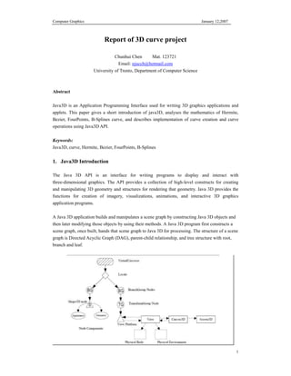
3. Scene Graph Structure

9
4. Implementation Detail
User Interface (package gui)
Class Functionality
CurveMain Main class for running application
Scene Initiate control and editor components
TextOutputPanel Display functionality status
CurveCtrls Curve control panel
Curve Editor (package editor)
Class Functionality
CurveEditor Curve editor panel, create java3d canvas
CurveGroup Wrap curve, points, and control lines.
Curve operations.
DrawerBehavior Curve drawing and operations
Curve Geometry (package curve)
Class Functionality
Curve Abstract class for curve geometry
HermiteCurve Hermite curve implementation
BezierCurve Bezier curve implementation
FourPointCurve FourPoints curve implementation
BsplineCurve B-Splines curve implementation
Utility (package util)
Class Functionality
ControlPoint Create control point geometry
ControlPointCallback Callback for changing point position
CurveCallback Callback for operating curve
Plane Create plane geometry for projection
GeomUtil Curve geometry utility
View
Class Functionality
Land Create land lines geometry
Curve Creation
Curve creation is based on the part of “Curve Mathematics” discussed above and implemented by
java. You can see details of implementation in accessory java document.
Curve Operation
As follows describe some main curve operations:

10
Project point on plane
If the application is in plane mode, create a plane with mouse clicking. While drawing curve, if the
mouse picking result is instance of Plane, we can get intersection point position on plane.
Cut
As curve is created by indexed coordinates, we can find the nearest curve coordinates from
clicking position.
Hermite curve:
Find two nearest curve coordinates, and make them as new curve’s startpoint and tangent of
startpoint. With these two new points and the other two, we can redraw new Hermite curve.
Other curves:
Find the nearest curve coordinate and index. Keep the line from first coordinate to found
coordinate, and delete the other.
Mirror
Find two nearest curve coordinates. Calculate the linear equation by these two coordinates. Then
mirror all of curve coordinates with that linear equation. At last, redraw the curve.
Bounding
Get curve bounds and create a box branch group with the bounds. Change curve branch group to
be a child of box transform group. Then the curve group is included in box branch group and can
be translated with it.
Copy
Pick selected curve and get all the parameters of picked curve. Create a new curve with the
parameters.
Join
Select the first curve, get the endpoint and the tangent of endpoint.
Select the second curve, get the startpoint and the tangent of startpoint.
Create a new Hermite curve, which the startpoint’s position and tangent equals to the endpoint’s
position and tangent of the first curve, the endpoint’s position and tangent equals to the startpoint’s
position and tangent of the second curve. The continuity is C1.
Save
Pick selected curve and get all the parameters of picked curve. Build a DOM with the parameters.
At last create an XML file from DOM and save it. On the contrary, to load a saved curve, just
parse all of elements in the saved XML file to get parameters of curve, then draw a curve with the
parameters in the scene graph.

11
5. Conclusion
In conclusion, this report gives an introduction of Java 3D, the mathematics of four different
curves, and describes the scene graph structure and also implementation details of project.
Through this project, we can understand the mathematics of parametric curves very well. The
implementation of this 3D curve application is a good experiment for advance 3D graphical
programming. A few of works can proceed based on this project in future.
Finally, thanks to Professor Raffaele De Amicis and Professor Conti for their guidance and help
through out the project.
Appendix (Application snapshot)

3D Curve Project

Recomendados

Recomendados

Mais conteúdo relacionado

Mais procurados

Mais procurados (20)

Destaque

Destaque (7)

Semelhante a 3D Curve Project

Semelhante a 3D Curve Project (20)

Mais de graphitech

Mais de graphitech (20)

Último

Último (20)

3D Curve Project