introdution to fluid mechanics

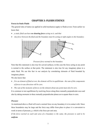
1. CHAPTER 3: FLUIDS STATICS
Forces in Static Fluids
The general rules of statics (as applied in solid mechanics) apply to fluids at rest. From earlier we
know that:
• a static fluid can have no shearing force acting on it, and that
• Any force between the fluid and the boundary must be acting at right angles to the boundary.
Pressure force normal to the boundary
Note that this statement is also true for curved surfaces; in this case the force acting at any point
is normal to the surface at that point. The statement is also true for any imaginary plane in a
static fluid. We use this fact in our analysis by considering elements of fluid bounded by
imaginary planes.
We also know that:
• For an element of fluid at rest, the element will be in equilibrium - the sum of the components
of forces in any direction will be zero.
• The sum of the moments of forces on the element about any point must also be zero.
It is common to test equilibrium by resolving forces along three mutually perpendicular axes and
also by taking moments in three mutually perpendicular planes an to equate these to zero.
Pressure
As mentioned above a fluid will exert a normal force on any boundary it is in contact with. Since
these boundaries may be large and the force may differ from place to place it is convenient to
work in terms of pressure, p, which is the force per unit area.
If the force exerted on each unit area of a boundary is the same, the pressure is said to be
uniform
1

2. Force
Pressure=
Area
Units: Newton’s per square metre, N m2, (The same unit is also known as a Pascal, Pa, i.e. 1Pa =
1 N m2) (Also frequently used is the alternative SI unit the bar, where 1bar =105 N m2)
Pascal’s Law for Pressure at a Point
(Proof that pressure acts equally in all directions.)
By considering a small element of fluid in the form of a triangular prism, which contains a point
P, we can establish a relationship between the three pressures px in the x direction, py in the y
direction and ps in the direction normal to the sloping face.
Triangular prismatic element of fluid
The fluid is a rest, so we know there are no shearing forces, and we know that all force are acting
at right angles to the surfaces .i.e.
ps acts perpendicular to surface ABCD,
px acts perpendicular to surface ABFE and
py acts perpendicular to surface FECD.
And, as the fluid is at rest, in equilibrium, the sum of the forces in any direction is zero.
(Please refer to pages 24 and 25 of Fluid Mechanics, Douglas J F, Gasiorek J M, and Swaffield J
A, Longman for the deivation)
px=py=ps
Pressure at any point is the same in all directions. This is known as Pascal’s Law and applies
to fluids at rest.
2

3. Variation of Pressure Vertically In a Fluid under Gravity
Vertical elemental cylinder of fluid
In the above figure we can see an element of fluid which is a vertical column of constant cross
sectional area, A, surrounded by the same fluid of mass density ρ . The pressure at the bottom of
the cylinder is p1 at level z1, and at the top is p2 at level z2. The fluid is at rest and in equilibrium
so all the forces in the vertical direction sum to zero.
i.e. we have
Force due to on A (upward) =p1A
Force due to on A (downward) =p2A
Force due to weight of element (downward) =mg= ρ Ag (z2-z1)
Taking upward as positive, in equilibrium we have
P1A- P2A- ρ Ag (z2-z1) = 0
P1- P2= ρ g (z2-z1)
Thus in a fluid under gravity, pressure decreases with increase in height z = (z2-z1)
Equality of Pressure at the Same Level in a Static Fluid
Consider the horizontal cylindrical element of fluid in the figure below, with cross-sectional area
A, in a fluid of density ρ , pressure Pl at the left hand end and pressure Pr at the right hand end.
3

4. Horizontal elemental cylinder of fluid
The fluid is at equilibrium so the sum of the forces acting in the x direction is zero.
PlA-PrA =0
Pl=Pr
Therefore, Pressure in the horizontal direction is constant.
This result is the same for any continuous fluid. It is still true for two connected tanks which
appear not to have any direct connection, for example consider the tank in the figure below.
Two tanks of different cross-section connected by a pipe
We have shown above that Pl=Pr and from the equation for a vertical pressure change we have
Pl=Pp+ ρ gz
and
Pr=Pq+ ρ gzr
Pp+ ρ gzr=Pq+ ρ gz
Pp=Pq
4

5. This shows that the pressures at the two equal levels, P and Q are the same.
General Equation for Variation of Pressure in a Static Fluid
Here we show how the above observations for vertical and horizontal elements of fluids can be
generalized for an element of any orientation.
A cylindrical element of fluid at an arbitrary orientation.
Consider the cylindrical element of fluid in the figure above, inclined at an angle θ to the
vertical, length ds, cross-sectional area A in a static fluid of mass density ρ . The pressure at the
end with height z is p and at the end of height z+ δz is p+ δp .
The forces acting on the element are
pA acting at right - angles to the end of the face at z
(p+ δp ) A acting at right - angles to the end of the face at z+ δz

Mg=A ρ δ sg the weight of the element acting vertically down
There are also forces from the surrounding fluid acting normal to these sides of the element. For
equilibrium of the element the resultant of forces in any direction is zero.
Resolving the forces in the direction along the central axis gives
pA-(p+ δp ) A - A ρ δ sgcos θ
 
5

6. δp
= - ρ gcos θ

δs
Or in the differential form
dp/ ds=- ρ gcos θ

If  θ =90, Then s is in the x or y directions, (i.e. horizontal), so
 dp   dp   dp 
   θ =90=   =   =0
  Confirming that pressure on any horizontal plane is zero.
 ds   dx   dy 
 dp   dp 
If  θ =0,_ then s is in the z direction (vertical) so    θ =0=   =- ρ g
 ds   dz 
Confirming the result
P2 − P1
= ρ g
Z 2 − Z1
P2- P1= ρ g (z2-z1)
Pressure and Head
 dp 
In a static fluid of constant density we have the relationship   =- ρ g, as shown above. This
 dz 
cans be integrated to give P=- ρ gz+ constant. In a liquid with a free surface the pressure at any

depth z measured from the free surface so that z = -h (see the figure below)
Fluid head measurement in a tank.
This gives the pressure p= ρ gh + constant
At the surface of fluids we are normally concerned with, the pressure is the atmospheric
pressure, p atmospheric . So p= ρ gh + patmospheric

6

7. As we live constantly under the pressure of the atmosphere, and everything else exists under this
pressure, it is convenient (and often done) to take atmospheric pressure as the datum. So we
quote pressure as above or below atmospheric.
Pressure quoted in this way is known as gauge pressure i.e. Gauge pressure is
pgauge = ρ gh
The lower limit of any pressure is zero - that is the pressure in a perfect vacuum. Pressure
measured above this datum is known as absolute pressure i.e.Absolute pressure is
pabsolute = ρ gh+ p atmospheric
Absolute pressure = Gauge pressure + Atmospheric pressure
As g is (approximately) constant, the gauge pressure can be given by stating the vertical height
of any fluid of density ρ which is equal to this pressure.
P= ρ gh
This vertical height is known as head of fluid.
Note: If pressure is quoted in head, the density of the fluid must also be given.
Example:
We can quote a pressure of 500K N m -2 in terms of the height of a column of water of density, ρ
=1000kg m-3 .
a) What is the pressure?
b) If the liquid was mercury with a density of 13.6x103kg m-3 what would be the head?
(Answers: 50.95m of water, 3.75m of Mercury)
Pressure Measurement by Manometer
The relationship between pressure and head is used to measure pressure with a manometer (also
known as a liquid gauge).
The Piezometer Tube Manometer
The simplest manometer is a tube, open at the top, which is attached to the top of a vessel
containing liquid at a pressure (higher than atmospheric) to be measured. An example can be
7

8. seen in the figure below. This simple device is known as a Piezometer tube. As the tube is open
to the atmosphere the pressure measured is relative to atmospheric so is gauge pressure.
A simple piezometer tube manometer
Pressure at A = pressure due to column of liquid above A
PA= ρ gh1
Pressure at B = pressure due to column of liquid above B
PB= ρ gh2
This method can only be used for liquids (i.e. not for gases) and only when the liquid height is
convenient to measure. It must not be too small or too large and pressure changes must be
detectable.
The “U”-Tube Manometer
Using a “U”-Tube enables the pressure of both liquids and gases to be measured with the same
instrument. The “U” is connected as in the figure below and filled with a fluid called the
manometric fluid. The fluid whose pressure is being measured should have a mass density less
than that of the manometric fluid and the two fluids should not be able to mix readily - that is,
they must be immiscible.
8

9. A “U”-Tube manometer
Pressure in a continuous static fluid is the same at any horizontal level so,
Pressure at B = pressure at C
PB=PC
For the left hand arm pressure at B = pressure at A + pressure due to height h1 of fluid being
measured 1
PB=PA + ρ gh1

For the right hand arm, pressure at C = pressure at D + pressure due to height h2 of manometric
fluid
PC=PAtmospheric + ρ mangh2
As we are measuring gauge pressure we can subtract PAtmospheric giving
PB=PC
PA= ρ mangh2- ρ gh1
If the fluid being measured is a gas, the density will probably be very low in comparison to the
density of the manometric fluid i.e. ρ man ρ . In this case the term ρ gh1 can be neglected,
and the gauge pressure is given by
PA = ρ mangh2
Measurement of Pressure difference using a “U”-Tube Manometer.
9

10. If the “U”-tube manometer is connected to a pressurized vessel at two points the pressure
difference between these two points can be measured.
B
A
Pressure difference measurement by the “U”-Tube manometer
If the manometer is arranged as in the figure above, then
Pressure at C = pressure at D
PC=PD
PC= PA+ ρ gha
PD= PB+ ρ g (hb-h) + ρ mangh
Giving the pressure difference
PA-PB= ρ g (hb-ha) + ( ρ man- ρ )gh
Again, if the fluid whose pressure difference is being measured is a gas i.e. ρ man ρ and then
the terms involving ρ can be neglected.
Advances to the “U” tube manometer.
The “U”-tube manometer has the disadvantage that the change in height of the liquid in both
sides must be read. This can be avoided by making the diameter of one side very large compared
10

11. to the other. In this case the side with the large area moves very little when the small area side
move considerably more.
Assume the manometer is arranged as above to measure the pressure difference of a gas of
(negligible density) and that pressure difference is P1-P2. If the datum line indicates the level of
the manometric fluid when the pressure difference is zero and the height differences when
pressure is applied is as shown, the volume of liquid transferred from the left side to the right
(
Z2X πd 2 / 4 )
And the fall in level of the left side is
Z1 =Volume moved/ Area of left side
( ) ( )
= Z2X πd 2 / 4 / ( πD 2 / 4 =Z2  d  2
 
D
We know from the theory of the “U” tube manometer that the height different in the two
columns gives the pressure difference so
 d 
2
  d 2 
P1-P2= ρ g  Z 2 + Z 2    == ρ gZ2 1 +    =

 D   D 
 
Clearly if D is very much larger than d then (d/D)2 is very small so P1-P2= ρ gZ2
So only one reading need be taken to measure the pressure difference. If the pressure to be
measured is very small then tilting the arm provides a convenient way of obtaining a larger
(more easily read) movement of the manometer. The above arrangement with a tilted arm is
shown in the figure below.
11

12. Tilted manometer.
The pressure difference is still given by the height change of the manometric fluid but by placing
the scale along the line of the tilted arm and taking this reading large movements will be
observed. The pressure difference is then given by
P1-P2= ρ gZ2= ρ gxsin θ
The sensitivity to pressure change can be increased further by a greater inclination of the
manometer arm; alternatively the density of the manometric fluid may be changed.
Choice of Manometer
Care must be taken when attaching the manometer to vessel; no burrs must be present around
this joint. Burrs would alter the flow causing local pressure variations to affect the measurement.
Some disadvantages of manometers:
• Slow response - only really useful for very slowly varying pressures - no use at all for
fluctuating pressures;
• For the “U” tube manometer two measurements must be taken simultaneously to get the h
value. This may be avoided by using a tube with a much larger cross-sectional area on
one side of the manometer than the other;
• It is often difficult to measure small variations in pressure - a different manometric fluid
may be required - alternatively a sloping manometer may be employed; It cannot be used
for very large pressures unless several manometers are connected in series;
12

13. • For very accurate work the temperature and relationship between temperature and must
be known;
Some advantages of manometers:
• They are very simple.
• No calibration is required - the pressure can be calculated from first principles.
Forces on Submerged Surfaces in Static Fluids
Fluid pressure on a surface
Pressure is defined as force per unit area. If a pressure p acts on a small area dA then the force
exerted on that area will be F =p δ A
Since the fluid is at rest, the force will act at right-angles to the surface.
General submerged plane
Consider the plane surface shown in the figure below. The total area is made up of many
elemental areas. The force on each elemental area is always normal to the surface but, in general,
each force is of different magnitude as the pressure usually varies.
We can find the total or resultant force, R, on the plane by summing up all of the forces on the
small elements i.e.
R= p1 δ A1+ p2 δ A2 +…+ pn δ An =∑ p δ A
This resultant force will act through the centre of pressure, hence we can say
If the surface is a plane the force can be represented by one single resultant force, acting at
right-angles to the plane through the centre of pressure.
13

14. Horizontal submerged plane.
For a horizontal plane submerged in a liquid (or a plane experiencing uniform pressure over its
surface), the pressure, p, will be equal at all points of the surface. Thus the resultant force will be
given by
R= pressure x area of plane
R =pA
Curved submerged surface
If the surface is curved, each elemental force will be a different magnitude and in different
direction but still normal to the surface of that element. The resultant force can be found by
resolving all forces into orthogonal co-ordinate directions to obtain its magnitude and direction.
This will always be less than the sum of the individual forces, ∑ p δ A
Resultant Force and Centre of Pressure on a submerged plane surface in a liquid.
This plane surface is totally submerged in a liquid of density  ρ and inclined at an angle of θ to
the horizontal. Taking pressure as zero at the surface and measuring down from the surface, the
pressure on an element dA , submerged a distance z, is given by
p = ρ gz and therefore the force on the element is
F= p δ A= ρ gz δ A
The resultant force can be found by summing all of these forces i.e.
R= ρ g ∑ z δ A (assuming ρ and g as constant).
14

15. The term ∑ z δ A is known as the 1st Moment of Area of the plane PQ about the free surface. It is
equal to A Z i.e. ∑ z δ A = A Z = 1st moment of area about the line of the free surface; where A
is the area of the plane and Z is the depth (distance from the free surface) to the centroid, G. This
can also be written in terms of distance from point O ( as Z = X sin θ )
∑ z δ A = A X sin θ , 1st Moment of area about a line through O X sin θ
The resultant force on a plane R= ρ gA Z = ρ gA X sin θ
This resultant force acts at right angles to the plane through the centre of pressure, C, at a depth
D. The moment of R about any point will be equal to the sum of the moments of the forces on all
the elements δ A of the plane about the same point. We use this to find the position of the centre
of pressure. The position of the centre of pressure along the plane measure from the point O is:
Σs 2δA
Sc= (Can be derived-look it up)
AX
It looks a rather difficult formula to calculate - particularly the summation term. Fortunately this
term is known as the 2nd Moment of Area, of the plane about the axis through O and it can be
easily calculated for many common shapes. So, we know:
2nd moment of area about O, I0 =∑s2 δ A

And as we have also seen that A X =1 st Moment of area about a line through O,thus the position
of the centre of pressure along the plane measure from the point O is:
S c = 2nd Moment of area about a line through O
1st Moment of area about a line through O
and the depth to the centre of pressure is
D= S c sin θ
How do you calculate the 2nd moment of area?
To calculate the 2nd moment of area of a plane about an axis through O, we use the parallel axis
theorem together with values of the 2nd moment of area about an axis though the centroid of the
shape obtained from tables of geometric properties.
The parallel axis theorem can be written
I0 =IGG+ A x 2
Where IGG is the 2nd moment of area about an axis though the centroid G of the plane.
15

16. Using this we get the following expressions for the position of the centre of pressure
I GG
Sc= +x
Ax
(In the examination the parallel axis theorem and the I GG will be given if necessary)
The second moment of area of some common shapes.
The table below gives some examples of the 2 nd moment of area about a line through the
centroid of some common shapes.
Lateral position of Centre of Pressure
If the shape is symmetrical, the centre of pressure lies on the line of symmetry. But if it is not
symmetrical its position must be found by taking moments about the line OG in the same way as
we took moments along the line through O
16

17. Submerged vertical surface - Pressure diagrams
For vertical walls of constant width it is usually much easier to find the resultant force and centre
of pressure. This is done graphically by means of a pressure diagram. Consider the tank in the
diagram below having vertical walls and holding a liquid of density ρ to a depth of H. To the
right can be seen a graphical representation of the (gauge) pressure change with depth on one of
the vertical walls. Pressure increases from zero at the surface linearly by p= ρ gz, to a maximum
at the base of p = ρ gH .
Pressure diagram for vertical wall.
The area of this triangle represents the resultant force per unit width on the vertical wall, using
SI units this would have units of Newtons per metre. So,
1
Area =  × AB × BC
2
1 1
= H ρ gH = ρ gH2
2 2
1
Resultant force per unit width = ρ gH2(N / m)
2
The force acts through the centroid of the pressure diagram. For a triangle the centroid is at 2/3
2
its height, i.e. in the figure above the resultant force acts horizontally through the point z = H
3
For a vertical plane the depth to the centre of pressure is given by
2
D= H
3
Resultant force on a submerged curved surface
17

18. As stated above, if the surface is curved the forces on each element of the surface will not be
parallel and must be combined using some vectorial method. It is most straightforward to
calculate the horizontal and vertical components and combine these to obtain the resultant force
and its direction. (This can also be done for all three dimensions, but here we will only look at
one vertical plane).
In the diagram below the liquid is resting on top of a curved base.
The element of fluid ABC is equilibrium (as the fluid is at rest).
Horizontal forces
Considering the horizontal forces, none can act on CB as there are no shear forces in a static
fluid so the forces would act on the faces AC and AB as shown below.
We can see that the horizontal force on AC, FAC, must be equal and be in the opposite direction
to the resultant force RH on the curved surface. As AC is the projection of the curved surface AB
18

19. onto a vertical plane, we can generalize this to say the resultant horizontal force of a fluid above
a curved surface is:
RH = Resultant force on the projection of the curved surface onto a vertical plane.
We know that the force on a vertical plane must act horizontally (as it acts normal to the plane)
and that RH must act through the same point. So we can say RH acts horizontally through the
centre of pressure of the projection of the curved surface onto a vertical plane. Thus we can use
the pressure diagram method to calculate the position and magnitude of the resultant horizontal
force on a two dimensional curved surface.
Vertical forces
The diagram below shows the vertical forces which act on the element of fluid above the curved
surface.
There are no shear forces on the vertical edges, so the vertical component can only be due to the
weight of the fluid. So we can say the resultant vertical force of a fluid above a curved surface is:
RV = Weight of fluid directly above the curved surface and it will act vertically downward
through the centre of gravity of the mass of fluid.
Resultant force
The overall resultant force is found by combining the vertical and horizontal components
vectorialy, Resultant force R= (R H
2
+ RV
2
) and acts through O at an angle θ .
The angle the resultant force makes to the horizontal is
19

20.  RV 
θ =tan-1  R
  

 H 
The position of O is the point of integration of the horizontal line of action of RH and the vertical
line of action of RV .
What are the forces if the fluid is below the curved surface? This situation may occur or a curved
sluice gate for example. The figure below shows a situation where there is a curved surface
which is experiencing fluid pressure from below.
The calculation of the forces acting from the fluid below is very similar to when the fluid is
above.
Horizontal force
From the figure below we can see the only two horizontal forces on the area of fluid, which is in
equilibrium, are the horizontal reaction force which is equal and in the opposite direction to the
pressure force on the vertical plane A’B. The resultant horizontal force, RH acts as shown in the
diagram. Thus we can say:
The resultant horizontal force of a fluid below a curved surface is:
RH =Resultant force on the projection of the curved surface on a vertical plane
20

21. Vertical force
The vertical force are acting are as shown on the figure below. If the curved surface were
removed and the area it were replaced by the fluid, the whole system would be in equilibrium.
Thus the force required by the curved surface to maintain equilibrium is equal to that force which
the fluid above the surface would exert - i.e. the weight of the fluid
Thus we can say:
The resultant vertical force of a fluid below a curved surface is:
Rv =Weight of the imaginary volume of fluid vertically above the curved surface.
The resultant force and direction of application are calculated in the same way as for fluids above
the surface:
Resultant force R= (R H
2
+ RV
2
)
And acts through O at an angle of θ
The angle the resultant force makes to the horizontal is
 RV 
θ =tan-1  R
  

 H 
21